
Advancements in CO2 Flux Estimation: 4-D Variational Data Assimilation Techniques
E N D
Presentation Transcript
Carbon Cycle Data Assimilation with a Variational Approach (“4-D Var”) David Baker CGD/TSS with Scott Doney, Dave Schimel, Britt Stephens, and Roger Dargaville 24 Sept 2004
Outline • The problem: estimate CO2 sources and sinks at fine space/time scales (2° x 2.5°, hourly/daily) • Method: • Why use 4-D Var? (Kalman) filtering, smoothing, and variational methods – pros and cons • Mathematical background of 4-D Var applied to atmospheric trace gases • Some 4-D Var results using simulated truth • Additional topics to ponder: • 100 descent iterations 100 ensemble members? • Error estimates: 4-D Var vs. ensemble filters
Transport: surface fluxes concentrations 0 H fluxes Transport basis functions concentrations
Present Future Shift towards newer instruments/platforms: • More continuous analyzers, new cheap in situ analyzers • Aircraft, towers (flux & tall), ships/planes of opportunity • CO2-sondes, tethered balloons, etc. • Satellite-based column-integrated CO2, maybe CO2 profiles Higher frequency with better spatial coverage -- will permit more detail to be estimated More sensitive to continental air, detailed flow features -- synoptic meteorology, diurnal cycle must be resolved Solve for the fluxes at the resolution of the transport model • 2° x 2.5°, 25 levels, daily/hourly time step • With current inversion techniques, computations grow as O(N3)… more efficient techniques required (iterative vs. direct inversions, adjoint allows efficient gradient computation, minimal storage)
For retrospective analyses, a 2-sided smoother gives more accurate estimates than a 1-sided filter. The 4-D Var method is 2-sided, like a smoother. (Gelb, 1974)
Variational Data Assimilation vs. Ensemble (Kalman) filter Pros: • Greater accuracy achieved with 2-sided smoother than 1-sided filter • Initial transients reduced Cons: • Adjoint model required • [Correlations are pre-specified, rather than calculated, as with a Kalman filter]
4-D Var Data Assimilation Method • Find optimal fluxes u and initial CO2 field xo to minimize • subject to the dynamical constraint • where • x are state variables (CO2 concentrations), • v are independent variables used in model but not optimized, • z are the observations, • R is the covariance matrix for z, • uo is an a priori estimate of the fluxes, • Puo is the covariance matrix for uo, • xo is an a priori estimate of the initial concentrations, • Pxo is the covariance matrix for xo
4-D Var Data Assimilation Method Adjoin the dynamical constraints to the cost function using Lagrange multipliers SettingF/xi = 0 gives an equation for i, the adjoint of xi: The adjoints to the control variables are given byF/uiandF/xooas: The optimal u and xo may then be found iteratively by
4-D Var Iterative Optimization Procedure 0 x0 ° Forward Transport Forward Transport Estimated Fluxes “True” Fluxes 1 2 Modeled Concentrations “True” Concentrations ° x1 ° Measurement Sampling Measurement Sampling x2 Modeled Measurements “True” Measurements Assumed Measurement Errors D/(Error)2 3 x3 ° Weighted Measurement Residuals Flux Update Adjoint Transport Adjoint Fluxes = Minimum of cost function J
Prior Truth OSSE fluxes, snapshot for Jan 1st Estimate (30 descent steps)
Prior - Truth Estimate - Truth
Future Plans for CO2 • Assimilate remotely-sensed data • Finer resolution (1º x 1º, or regional) • Improve predictive capability of carbon cycle models (in two steps) by • Tying fluxes to remotely-sensed patterns • Estimating parameters in ocean and land biosphere models using remotely-sensed fields directly as data
Atmospheric transport model NASA/GSFC DAO ‘PCTM’ model: • Lin-Rood advection • Vertical diffusion • Simple cloud convection • Driven by saved wind & mixing fields from DAO analyses • 6-hourly winds interpolated to 15 minute time step • 2º x 2.5º resolution, 25 vertical levels Adjoint: • Coded manually; straight-forward because of • Linearity of CO2 transport • Simplicity of vertical mixing routines • Runs as fast as forward code