Download
1 / 5
0 likes | 7 Views
Solution Manual for Linear and Convex Optimization: A Mathematical Approach<br>Author: Michael H. Veatch<br>https://solumanu.com/product/linear-and-convex-optimization-veatch/<br><br>Explore the principles of linear and convex optimization with this solution manual. It provides clear, methodical solutions to key problems, supporting students in mastering the subjectu2019s fundamental concepts.<br>The Solution manual is in PDF format and has 124 pages totally

E N D
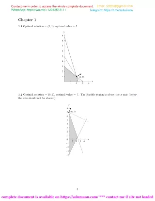
Email: smtb98@gmail.com Telegram: https://t.me/solumanu Contact me in order to access the whole complete document. WhatsApp: https://wa.me/+12342513111 Chapter 1 1.1 Optimal solution = (2,1), optimal value = 5 y 9 8 7 6 5 4 3 2 1 (2, 1) x 1 2 3 4 1.2 Optimal solution = (0,7), optimal value = 7. The feasible region is above the x-axis (below the axis should not be shaded). y 8 (0, 7) 7 6 5 4 3 2 1 x 0 1 2 3 4 –1 –2 –3 –4 3 complete document is available on https://solumanu.com/ *** contact me if site not loaded
Contact me in order to access the whole complete document. WhatsApp: https://wa.me/+12342513111 smtb98@gmail.com Email: smtb98@gmail.com Telegram: https://t.me/solumanu 1.3 Optimal solutions: the line segment from (90,20) to (662 smtb98@gmail.com 3,662 3), optimal value = 3000 y 300 250 200 150 100 (66⅔, 66⅔) 50 (90,20) x 50 100 150 200 1.4 a) Optimal solution = (100,200), optimal value = 400. b) Unbounded. Sweeping the objective function line in the opposite direction to that in (a), the line never leaves the feasible region. y 300 (100,200) 200 100 x 300 100 200 4 complete document is available on https://solumanu.com/ *** contact me if site not loaded
1.5 Infeasible. The region satisfying constraints 1 and 3 does not intersect the nonnegative quad- rant, so there are no feasible solutions. y 5 3 4 3 1 2 1 x 2 4 6 8 10 12 14 –1 –2 1.6 Optimal integer solution = (2,3), optimal value = 18. The optimal solution lies on the first constraint. y 7 6 5 4 3 (2, 3) 2 1 x 1 2 3 4 5 6 5 complete document is available on https://solumanu.com/ *** contact me if site not loaded
smtb98@gmail.com 1.7 Optimal integer solution = (1,7), optimal value = 10. The optimal solution is at the intersection of constraints 2 and 3. smtb98@gmail.com y 9 8 (1, 7) 7 6 5 4 3 2 1 x 1 2 3 4 5 6 7 8 1.8 Optimal integer solution = (1,3), optimal value = 17. The optimal solution does not lie on any of the constraints. y 7 6 5 4 3 (1, 3) 2 1 x –3 –2 –1 1 2 3 4 1.9 a) Optimal solution = (0,0), i.e., send no aid. There are no constraints requiring aid to be sent. b) Any objective maxc1x + c2y, where c1,c2 > 0 and c1 < c2. For example, maxx + 2y. The contour line x + 2y = 11 touches the feasible region only at (1,5), showing that it is optimal. 6 complete document is available on https://solumanu.com/ *** contact me if site not loaded
Chapter 2 2.1 Let U = number of Ultimate produced P = number of Pool produced D = number of Discs produced Add the constraints U ≥ 3500, P ≥ 1000, D ≥ 2800, P ≤ 0.25(U + P) Remove the constraint P ≤ 2000 Optimal solution: U = 3900, P = 1300, D = 2800, profit = $60,200 2.2 Let xj = batches of part j produced. Remove the drilling and polishing constraints and add the constraint 6x1+ 3x2+ 4x3+ 4x4≤ 500 (drilling and polishing) Optimal solution: x = (70,10,10,10), profit = $10,200. Profit increases because cross-training expands the feasible region. 2.3 a) Let A = units of product A produced B = units of product B produced max (54 − 7.2)A + (48 − 5.4)B s.t 1.5A + 0.75A + 2B ≤ 900 (assembly) 2B ≤ 800 (packaging) A,B ≥ 0 Optimal solution: A = 600, B = 0, profit = $28,080 b) Let y = additional assembly labor (hrs) max (54 − 7.2)A + (48 − 5.4)B − 15y s.t 1.5A + 0.75A + 2B − 2B y ≤ 900 (assembly) ≤ 800 (packaging) y ≤ 300 A,B,y ≥ 0 Optimal solution: A = 800, B = 0, y = 300 hours, profit = $32,940 2.4 Let xj= number of type j surgeries per week max 14x1+ 10.5x2+ 3.5x3+ 2.1x4 s.t. 7x1+ 4x2+ 5x1+ 2x2+ 30x1+ 10x2+ x1 x1≥ 10,x2≥ 10,x3≥ 20,x4≥ 0 (profit in $1000s) x4≤ 2x3+ x3 5x3+ 456 800 (OR) ≤ (bed days) (nurse) x4≤ 40,000 ≤ 25 (type 1 demand) 7 complete document is available on https://solumanu.com/ *** contact me if site not loaded