Download
1 / 57
570 likes | 792 Views
Chapter 4 Discrete Random Variables 4.1 Discrete and Continuous 4.2 Probability Distribution 4.3 Expectation and Variance 4.4 Binominal 4.5 Poisson 4.6 Hypergeometric Homework: 3,5,7,9,11,13,15,21,23,27,31, 43,52,53,61,63,68,69,77.

E N D
Chapter 4 Discrete Random Variables 4.1 Discrete and Continuous 4.2 Probability Distribution 4.3 Expectation and Variance 4.4 Binominal 4.5 Poisson 4.6 Hypergeometric Homework: 3,5,7,9,11,13,15,21,23,27,31, 43,52,53,61,63,68,69,77 1
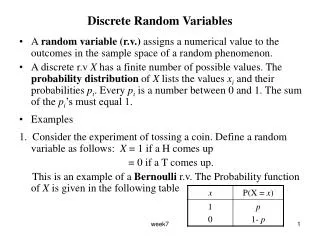
Last chapter we discussed several useful concepts of dealing with probability problems. However, it is very difficult to write down sample spaces of some random experiments. In these cases the concept random variable is very useful. A random variable is a variable that assumes values associated with the random outcomes of a random experiment, where one and only one numerical values is assigned to each sample point. It is random because we can not predict the outcome of a random experiment. It is a variable because there are more than one possible sample points in a random experiment. 2
<Example 4.1>: (Basic) One hundred fair coins are tossed and the up faces are observed. (a) Is it convenient to write down the sample space for this random experiment? (b) Do we need to write down the sample space if we are interested in counting the number of heads in this random experiment? <Solutions>: (a) No, it takes vary long time to write the sample space of this random experiment. (b) No, we can use the concept of random variable to solve our problem. 3
Section 4.1: Discrete and Continuous Random Variable Some random variable can assume values on countable many numbers (such as integers) and some random variable can assume values on one or more intervals. For example, the distance between you home and UCF is between 0 and 100 miles that is an interval, i.e. the distance between your home and UCF is a continuous random variable. But the number of head in coin tossing experiment is a countable number, i.e. the number of heads in a coin tossing experiment is a discrete random variable. 4
<Example 4.2> (Basic) List five discrete random variables and five continuous random variables. 5
Sec 4.2: Probability Distributions for Discrete Random Variables This chapter will focus on the discussion of discrete random variable. A complete description of a discrete random variable requires that we specify all the possible values the random variable can assume and the probability associated with each value. Usually, we can use the following four steps to complete a probability table. Step 1: Find out the variable of interest. Step 2: List all the sample points in the sample space. Step 3: List all the possible values of this random variable. Step 4: Assign the probabilities to all the possible values. 6
<Example 4.3>: (Basic) A company has five applicants for two positions: three from UCF and two from UF. Suppose that the five applicants are equally qualified and no preference is given for choosing either school. Let x be the number of UCF graduates chosen to fill the two positions. (a) What is the random variable of interest? (b) Write down the sample space. (c) Write the probability table. 7
The probability distribution of a discrete random variable is a graph, a table, or a formula that specifies the probability associated with each possible value the random variable can assume. The probability distribution should not include values that have zero probabilities. The rules to assign probability discussed in Section 3.2 should be followed as well. Thus, the probability of any value of a random variable is between 0 and 1 and the sum of the probabilities of all possible values of a random variable is equal to one. 8
<Example 4.4>: (Basic) A random variable has the following probability table: x 0 1 2 3 4 p(x) 0.1 0.2 0.3 ? 0.15 (a) Find P(x=3). (b) Is x a continuous random variable? 9
<Example 4.5>: (Advance) A lady claims that she can taste the difference between PEPSI and COKE. Therefore, we conduct an experiment to confirm her claim. Four cups of cola that some are COKE colas and some are PEPSI colas are displayed in front of her. After tasting these colas, she needs to identify the contents in each cups. We are interested in the correct decisions made by her in this experiment. (a) What is the random variable of interest? (b) Write down the sample space. (c) Write the probability table. 10
Sec 4.3: Expectation and Variance of a Discrete Random Variable We discussed how to obtain the sample mean, the sample variance, and the sample standard deviation in chapter 2. Now, we introduce the formulas of getting the population mean, the population variance, and the population standard deviation of a discrete random variable. Suppose X is a discrete random variable with probability distribution p(x). The expectation of X is the population mean of X. Let m, , and s be the population mean, the population variance, and the population standard deviation of X, respectively. Then m = E(x) = S xp(x), s2= E[(x-m)2] = S (x-m)2 p(x), and 11
<Example 4.6>: (Basic) Consider the probability table of random variable x below. x p(x) 1 0.1 3 0.2 5 0.3 6 0.3 10 0.1 12
(a) Find the expectation of this random variable. <Solution>: x p(x) xp(x) 1 0.1 0.1 3 0.2 0.6 5 0.3 1.5 6 0.3 1.8 10 0.1 1.0 mean = m = Sxp(x) = 0.1 + 0.6 + 1.5 + 1.8 + 1.0 = 5 13
(b) Find the standard deviation of this random variable. <Solution>: x-m (x-m)2 (x-m)2p(x) -4 16 1.6 -2 4 0.8 0 0 0 1 1 0.3 5 25 2.5 the variance = =S p(x) = 1.6+0.8+0+0.3+2.5=5.2 and the standard deviation = s = 2.28. 14
(c) What is the probability that x falls within the interval (m-2s, m+2s)? (d) Does the result satisfy the Chebyshev’s Rule? (e) Does the result satisfy the Empirical Rule? Explain. <Solutions>: (c) m-2s = 5 - 2*2.28 = 0.44 m+2s = 5 + 2*2.28 = 9.56 Thus, the probability that x falls within the interval (m-2s, m+2s) is 0.9 (0.9=0.1+0.2+0.3+0.3). (d) Yes. (e) No, because the random variable x does not have a mound-shape distribution. 15
<Example 4.7>: (Basic) You need to pay one dollar to buy an instant lottery ticket. In this instant lottery game, you have 10% chance to win a one dollar bill and 5% chance to win a five dollar bill. You are interested in the money which you can win in a single play. 16
(a) Write down the probability table. <Solution>: x p(x) 1 0.1 5 0.05 0 0.85 Note: The lottery official does (not?) want you to know that you have 85% chance to “win” nothing. 17
(b) Find the mean. <Solution>: x p(x) xp(x) 1 0.1 0.1 5 0.05 0.25 0 0.85 0 mean = m = Sxp(x) = 0.1+0.25+0 = 0.35 18
(c) Find the standard deviation of the game. <Solution>: x-m (x-m)2 (x-m)2p(x) 0.65 0.4225 0.04225 4.65 21.6225 1.081125 -0.35 0.1225 0.104125 the variance = s**2 = S (x-m)**2 p(x) = 0.04225+1.081125+0.104125 = 1.2275 and the standard deviation = s = 1.10793. 19
(d) Do you believe the lottery officials claim ``the more you play the more you win’’? <Solution>: Clearly, I don’t believe it because lottery revenue is another form of taxes for the lottery players. 20
<Example 4.8>: (Basic) A study selected a sample of fifth grade pupils and recorded how many years of school they eventually completed. Let X be the highest year of school that a randomly selected fifth grader completes. (Students who go on to college are included in the outcome of x=12.) The probability is as follows: x 4 5 6 7 8 9 10 11 12 p(x) .01 .007 .007 ? .032 .068 .070 .041 .752 (a) Find P(X = 7). <Solution>: P(X=7)=1-(0.01+0.007+0.013+0.032+ 0.068+0.070+0.041+0.752) = 0.007. 21
(b) Find the mean and standard deviation. <Solutions>: x p(x) x * p(x) (x-m)2 (x-m)2p(x) 4 0.01 0.04 52.577001 0.52577001 5 0.007 0.035 39.075001 0.273525007 6 0.007 0.042 27.573001 0.193011007 7 0.013 0.091 18.071001 0.234923013 8 0.032 0.256 10.569001 0.338208032 9 0.068 0.612 5.067001 0.344556068 10 0.070 0.700 1.565001 0.10955007 11 0.041 0.451 0.063001 0.002583041 12 0.752 9.024 0.561001 0.421872752 11.251 2.44400 Thus, m=11.251, s2 = 2.44400, and s = 1.563. 22
(c) Find P(x >= 9). (d) Can you apply the Empirical rule to find the probability of X falls into the interval (m-2s, m+2s)? <Solutions>: (c) P(X 9) = .068+.070+.041+.762 = 0.931 (d) m-2s = 11.251 - 2* 1.563 8.124 m+2s = 11.251 + 2 * 1.563 14.378 Thus, the probability that x falls within the interval (m-2s, m+2s) is 0. 934. Although the probability is close to 0.95, we can only apply the chebyshev’s Rule because the empirical distribution of this random variable is not mound-shape. 23
Sec 4.4: The Binomial Random Variable The responses of many experiments have only two alternatives such as "Yes or No”, "True or False", "Male or Female”, and "Failure or Success". These types of experiments have some characteristic in common. First, they consist of n identical and independent trials. Second, there are only two possible outcomes, denoted by S and F on each trail. Third, the possibility of each outcome remains unchanged from trial to trial, that is, the probability of S is p and probability of F is q=(1-p) in each trial. 24
Fourth, we are interested in the random variable x represented the number of S happened in n trails (n is a fixed number). Therefore, it is worth to develop a special probability model to deal with this kind of random variables. Any random variable that has these four characteristics is called binomial random variable and can be dealt with by using this special probability model. 25
<Example 4.9>: (Basic) List several random variables that have only two possible outcomes. <Solutions>: Gender of a student in STA 3023; Win or Loss in a football game; Pass or Fail in an exam; Hit or Miss in a state lottery drawing; True or False to answer a question; 26
<Example 4.10>: (Basic)For each of the following situations, indicate whether a binomial distribution is a reasonable probability model for the random variable X. (a) A couple decides to continue to have children until their first girl is born; X is the total number of children the couple has. (b) Fifty students are taught about binomial probabilities by a television program. After completing their study, all students take the same examination; X is the number of students who passed this exam. (c) A chemist repeats a solubility test 10 times on the same substance. Each test is conducted at a temperature 10 degrees higher than the previous test. 27
Suppose that X is a binomial random variable. The probability of success on any single trial is p and there are n trials in this random experiment. The probability density function of X is where p = the probability of success on any single trial n = total number of trials q = 1 - p x = number of successes in n trials. 28
Let m and s be the mean and standard deviation of the binomial random variable X. In stead of using the expectation summation rules to calculate m and s, we can find m and s easily using the formulas m = np, s**2 = npq = np(1-p),and 29
<Example 4.11>: (Basic) To test the side effect of a newly developed medicine, we conduct an animal experiment. Five dogs are given this drug and each dog has 20% chance to develop certain symptoms. We are interested in the number of dogs that develop this symptom. (a) Is this a binomial random variable? 30
(b) Write down the probability table of this random variable. <solution to part (b)>: Probability Table: X P(X=x) 0 0.32768 1 0.4096 2 0.2048 3 0.0512 4 0.0064 5 0.00032 31
(c) Find the mean and standard deviation of this random variable. <solution to part (c)>: m = np = 5 * 0.2 = 1; s**2 = npq = 5 * 0.2 * 0.8 = 0.8; s = 0.894. 32
<Example 4.12>: (Basic) A firm receives a shipment of 500 hi-fi speakers. For any randomly selected sample of 9 speakers, if 2 or more of the speakers are defective then rejects this shipment. What is the probability that this firm will accept the shipment if the proportion of defective is (a) 0.20. (b) 0.10. (c) 0.05. 33
<Example 4.13>: (Basic) An oil exploration firm plans to drill six holes. Due to experience, the probability of each hole yielding oil is 0.12. Since the holes are in quite different locations, the outcome of drilling one hole is statistically independent of drilling of any other holes. (a) Give the expectation and standard deviation of the number of holes that results in oil. <Solution to part (a)>: (a) n = 6 and p = 0.12; m = np = 6 * 0.12 = 0.72; s = = 0.796; 34
(b) If the firm will be able to stay in business only if two or more holes produce oil, what is the probability that it can survive. <Solution to part (b)>: P(X ³ 2) = P(X=2) +(X=3)+P(X=4)+P(X=5)+ P(X=6) = 0.129534197 +0.023551672+ 0.00240869376+0.000131383296 +0.000002985984 @ 0.156 35
Note: (1) We can not use the Binomial probabilities Table to obtain this probability because p = 0.12 is not in the Table. (2) We can obtain this probability much easier with the concept of complement event: P(X 2) = 1 - P(X1) = 1 - P(X=0) - P(X=1) = 1 - 0.4644044086 - 0.37996698 @ 0.156 36
Section 4.5: The Poisson Random Variable The random variables produced by many random experiments can be well described by using Poisson probability model. Typical examples are as follows: (1) the number of customers served per hour in a given restaurant, (2) the number of alcohol related traffic accidents per month at a busy intersection, (3) the number of diseased trees per acre in a certain national park, (4) the number of telephone calls received per minute during your lunch hour. 37
Poisson random variable has the following common characteristics. (1). The experiment consists of counting the number of times that a certain event occurs during a given unit of time or in a given area or volume. (2). The probability of an event occurs in a given unit of time is same for all time units. (3). The number of events that occur in one unit of time, area, or volume is independent of the number that occur in other units. 38
The probability density function of a Poisson random variable is Both the mean and the variance of a Poisson random variable equals to l, i.e. m = l and s2 = l. 39
<Example 4.14>: (Basic) Suppose x is a Poisson random variable, use Table III on page 804 to find the following probabilities. (a) P(x £2) when l = 1. <Solution to part (a)>: part of Table III x =0 1 2 3 4 5 6 l = 1 .368 .736 .920 .981 .996 .999 1.000 Thus, P(X£2) = 0.920. 40
(b) P(x ³ 2) when m = 2. <Solution to part (b)> part of Table III x =0 1 2 3 4 5 6 7 8 l=2 .135 .406.677 .857 .956 .987 0.997 0.999 1.000 Since l = m = 2, P(x ³ 2) = 1 - P(x £ 1) = 1 - 0.406 = 0.594. 41
(c) P(x >3) where s2 = 3. <Solution to part (c)>: part of Table III x=0 1 2 3 4 5 6 7 8 l=3 0.050 0.199 0.423 0.647 0.815 0.916 0.996 0.988 0.996 Since s2 = m = 3, P(x > 3) = 1 - P(x £ 2) = 1 - 0.423 = 0.577. 42
Note: For Poisson random variable, we can find P(x £ a) from the table directly if a is an integer. We need to apply the concept of complement event to find the probability of P(x > a) or P(x ³ a). We need to know that P(x > a) = 1 - P(x £ a) and P(x ³ a ) = 1 - P(x £ a-1). 43
<Example 4.15>: (basic) We know that the mean of a Poisson random variable is equal to 2. Find the probabilities of x equal to 1, 2, and 3. <Solutions>: We can use the probability function to compute the probability of a Poisson random variable as well. 44
<Example 4.16>: (Intermediate) According to the records of an airline, the number of people who buy tickets but fail to show up for the early morning flight between Orlando and Washington D.C. is a Poisson random variable. We know that the standard deviation of this random variable is 2. Determine the probabilities that the number of no shows in an early flight (a) is equal to 5, (b) is less than or equal to 3, (c) is greater than or equal to 6. 45
<Solutions to EX 4.16>: l = s2 = 2 * 2 = 4 (a) (b) p(x £ 3) = 0.433. (From Table III) (c ) p(x³6) = 1 - p(x£5) = 1 - 0.785 = 0.215. 46
Section 4.6 The Hypergeometric Random Variable Hypergeometric random variableis another popular discrete random variable. Suppose there are a total of N balls: r red balls and (N-r) white balls, in a bag. And n balls are randomly selected from this bag without replacement. Let X denote the number of red balls in the n balls selected. Then the distribution of X is called a Hypergeometric distribution, with parameters N, r and n. 47
The probability density function of this hypogeometric distribution is given by: 48
<Example 4.17>: (Basic)Given that x is a hypergeometric random variable, compute p(x), m, and s**2 for each of the following cases: (a) N=5, n=3, r=3, x=1. <Solutions>: 49
(b) N=9, n=5, r=3, x=3. <Solution to part (b)>: 50