Download
1 / 24
491 likes | 975 Views
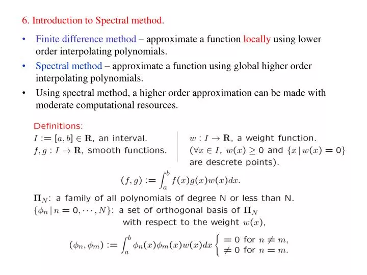
6. Introduction to Spectral method. Finite difference method – approximate a function locally using lower order interpolating polynomials. Spectral method – approximate a function using global higher order interpolating polynomials.

E N D
6. Introduction to Spectral method. • Finite difference method – approximate a function locally using lower order interpolating polynomials. • Spectral method – approximate a function using global higher order interpolating polynomials. • Using spectral method, a higher order approximation can be made with moderate computational resources.
In spectral methods, a function f(x) is approximated by its projection to the polynomial basis • Difference between f(x) and the approximation PNf(x) is called the truncation error. For a well behaved function f(x), the truncation error goes to zero as increasing N. Ex) an approximation for a function u(x) = cos3(p x/2) – (x+1)3/8
Gaussian integration (quadrature) formula is used to achieve high precision. • Gauss formula is less convenient since it doesn’t include end points of I = [a,b].
Gauss-Lobatto formula. • Since we have two less free parameters compare to the Gauss formula, the degree of precision for the Gauss-Lobatto formula is D = 2N – 1. • Since N – 1 roots are used for { xi }, the basis is • For I = [-1,1] and w(x) = 1, xi are roots of fN-1 = P’N(x)=0.
``Exact’’ spectral expansion differs from numerically evaluated expansion. • The Interpolant of f(x), IN f , is called the spectral approximation of f(x). • Abscissas used in the Gauss quadrature formula {xi} are also called collocation points. Exc 6-1) Show that the value of interpolant agrees with the function value at each collocation points,
A set of function values at collocation points • is called configuration space. • A set of coefficients of the spectral expansion • is called coefficient space. The map between configuration space and coefficient space is a bijection (one to one and onto). Ex) a derivative is calculated using a spectral expansion in the coefficient space.
Error in interpolant. Error in derivative.
Choice for the polynomials: 1) Legendre polynomials. fn(x) = Pn(x). Interval I = [-1,1], and weight w(x) = 1.
Some linear operations to the Legendre interpolant. Exc 6-2) Show the above relations using recursion relations for Pn(x).
2) Chebyshev polynomials. fn(x) = Tn(x). Interval I = [-1,1], and weight
Some linear operations to the Chebyshev interpolant. Exc 6-3) Show the above relations using recursion relations for Tn(x).
Convergence property For C1 – functions, the error decays faster than any power of N. (evanescent error)
Differential equation solver. Consider a system differential equations of the following form. Land B are linear differential operators. Numerically constructed function is called admissible solution, if i.e. satisfies boundary condition exactly, and Weighted residual method requires that, for N+1 test functions xn(x)
Recall: Notation for the spectral expansion. Gauss type quadrature formula (including Radau, Lobatto) is used. Continuum.
Three types of solvers. • Depending on the choice of the spectral basis fn and the test function xn, one can generate various different types of spectral solvers. • A manner of imposing boundary conditions also depend on the choice. • The Tau-method. • Choose fn as one of the orthogonal basis such as Pn(x), Tn(x). • Choose the test function xn the same as the spectral basis fn . • The collocation method. • Choose fn as one of the orthogonal basis such as Pn(x), Tn(x). • Choose the test function xn = d ( x – xn ) fpr any spectral basis fn. • The Galerkin method. • Choose the spectral basis fn and the test function xn as some linear combinations of orthogonal polynomial basis Gn that satisfies the boundary condition. The basis Gnis called Galerkin basis. • ( Gnis not orthogonal in general. )
The Tau-method. • Choose the test function xn the same as the spectral basis fn . Then solve (Note: here we have N+1 equations for N+1 unknowns.) • Linear operator, L, acting on the interpolant • can be replaced by a matrix Lnm . Therefore becomes • A few of these equations with the largest n are replaced by the • boundary condition. (The number is that of the boundary condition.)
The Tau-method (continued). • Boundary condition: suppose operator on the boundary B is linear,
A test problem. Consider 2 point boundary value problem of the second order ODE, • This boundary value problem • has unique exact solution, Example: Apply Tau-method to the test problem with the Chebyshev basis.
Example: Apply Tau-method to the test problem with the Chebyshev (Continued) The spectral expansion of the R.H.S becomes Boundary conditions Replace two largest componets (n = 4 and 3) of with the two boundary conditions. Done!
The collocation method. • Choose fn as one of the orthogonal basis such as Pn(x), Tn(x). • Choose the test function xn = d ( x – xn ) fpr any spectral basis fn. • Then solve, This is rewritten , or, Note the difference from the Tau method. LHS double sum. RHS not a spectral coefficients The boundary points are also taken as the collocation points. (Lobatto) The equations at the boundaries are replaced by the boundary conditions. Ex). A test problem with Chebyshev basis. Exc 6-4) Make a spectral code to solve the same test problem using the collocation method. Try both of Chebyshev and Legendre basis. Estimate the norm ||IN f – f || for the different N.
The Galerkin method. • Choose the spectral basis fn and the test function xn as some linear combinations of orthogonal polynomial basis Gn that satisfies the boundary condition. The basis Gnis called Galerkin basis. – The Galerkin basis is not orthogonal in general. – It is usually better to construct Gn that relates to a certain orthogonal basis fn in a simple manner (no general recipe for the construction.) Ex) – Highest order of the basis should be N – 1 to maintain a consistent degree of approximation. (so the highest basis appears is TN(x) . )
Ex) Consider the case with two point boundary value problem. Number of collocation points is N + 1. Since two boundary condition is imposed on the Galerkin basis {Gn} {Gn}: N – 1 are basis, n= 0, …, N – 2 . Assume that {Gn} can be constructed from a linear combination of the orthogonal basis {fn}. Then we may introduce a matrix Mmn such that The interpolant is defined by Taking the test function xn the same as Galerkin basis Gn , Exc 6-5) Show that this equation is wrtten Finally, using transformation matrix Mmn again, we spectral coefficients