CHAPTER 3 Forecasting
CHAPTER 3 Forecasting. Outline. Definition Forecast Accuracy Types of Forecasts Judgmental Time series Associative models. Forecast. A statement about the future value of a variable of interest, such as demand. Equivalently, prediction about the future.

CHAPTER 3 Forecasting
E N D
Presentation Transcript
Outline • Definition • Forecast Accuracy • Types of Forecasts • Judgmental • Time series • Associative models
Forecast A statement about the future value of a variable of interest, such as demand. Equivalently, prediction about the future. - Not necessarily numerical, e.g. weather forecasts
Cautions • Assume a causal system • Future resembles the past • Forecasts rarely perfect because of randomness • Forecasts more accurate for groups vs. individuals. • Forecasting errors among items in a group usually have a canceling effect. • Extremes in a group cancel each other • Forecast accuracy decreases as time horizon for forecasts increases. • Ex. weather forecast
“The forecast” Step 6. Monitor the forecast Step 5. Make the forecast Step 4. Obtain, clean, analyze appropriate data Step 3. Select a forecasting technique Step 2. Establish a time horizon Step 1. Determine purpose of forecast Steps in the Forecasting Process
Forecast Error • Error: Difference between the actual value and the value that was predicted for a given period. Errort= Actualt- Forecastt
Actualt Forecastt MAD = n ( Actualt Forecastt) MSE = n - 1 Actualt Forecastt × 100 Actualt MAPE = n Measures of Forecast Accuracy • Mean Absolute Deviation (MAD) • Mean Squared Error (MSE) • Mean Absolute Percent Error (MAPE) 2
Period Forecast (A-F) |A-F| (A-F) 2 1 215 2 216 3 215 4 214 5 211 6 214 7 217 8 216 Example 1 (|A-F|/Actual)×100 Actual 217 213 216 210 213 219 216 212
(|A-F|/Actual)×100 Period Forecast (A-F) |A-F| (A-F) 2 1 215 2 2 4 0.92 2 216 -3 3 9 1.41 3 215 1 1 1 0.46 4 214 -4 4 16 1.90 5 211 2 2 4 0.94 6 214 5 5 25 2.28 7 217 -1 1 1 0.46 8 216 -4 4 16 1.89 -2 22 76 10.26 Example 1 Actual 217 213 216 210 213 219 216 212 MAD= ׀A-F׀/ n = 22 / 8 = 2.75 (A-F)2/ (n-1) = 76 / 7 = 10.86 MSE = 10.26/8 = 1.28 MAPE =
Types of Forecasts • Judgmental - uses subjective inputs • Executive opinions • Sales force opinions • Consumer surveys • Time series - uses historical data assuming the future will be like the past • Associative models - uses explanatory variables to predict the future
Time series • Time-ordered sequence of observations taken at regular intervals • Data : measurements of demand (sales, earnings, profits, …) • Example: • Types of Variations in Time Series Data: • Trend - long-term movement in data • Seasonality - short-term regular variations in data • Cycles - wavelike variations of long-term • Irregular variations - caused by unusual circumstances • Random variations - caused by chance
Forecast Variations Irregularvariation Trend Cyclical Cycles Year 01 00 99 Seasonal variations
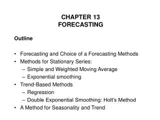
Time Series Methods • Naïve methods • Moving average • Weighted moving average • Exponential smoothing • Forecasting with a trend • Forecasting with seasonality
Time Series Forecasting - Naïve Method
Naïve Forecast Uh, give me a minute.... We sold 250 wheels last week.... Now, next week we should sell.... The forecast for any period = The previous period’s actualvalue.
Naïve Method Some Notation: Today’s temperature is 63 → AToday= 63 Forecast for tomorrow → FTomorrow= 63
1 2 3 4 5 6 7 8 9 10 11 12 42 40 43 40 41 39 46 44 45 38 40 - Example 2: Naïve Forecasts • Forecast for periodt is the actual value for period t-1: Ft = At-1.
Solution to Example 2 1 2 3 4 5 6 7 8 9 10 11 12 42 40 43 40 41 39 46 44 45 38 40 - - 42 40 43 40 41 39 46 44 45 38 40
Time Series Forecasting - Averaging
Ft = MAn= n Where t = an index that corresponds to periods. n = Number of periods (data points) in the moving average period. At = Actual value in period t. MAn = Forecast based on most-recent n periods. Ft = Forecast for time period t. n At-i i = 1 Moving Average • Moving average – A technique that averages a number of recent actual values, updated as new values become available.
1 2 3 4 5 6 7 8 9 10 11 12 42 40 43 40 41 39 46 44 45 38 40 - Example 3: Moving Average • Find moving average with n = 5.
42+40+43+40+41 = 5 46+44+45+38+40 = 5 Solution to Example 3 • Start from F6 (forecast for period 6). 1 2 3 4 5 6 7 8 9 10 11 12 42 40 43 40 41 39 46 44 45 38 40 - - - - - - 41.2 40.6 41.8 42.0 43.0 42.4 42.6
Moving Averages • New value becomes available? • Drop oldest value from total • Add newest value to total • Recalculate average (divide by n)
Lag Increases with Periods MA3 Average the last 3 actual values MA5 Average the last 5 actual values
Moving Averages • Fewer data points(n ) • More responsive to real changes • More responsive to random variations
1 wi= n At-i n 1 i = 1 MAn = = At-i n n i = 1 Weighted Moving Averages Weighted moving average – more recent values in a series are given more weight in computing the forecast Reminder that Simple Moving Average: n Ft = WMAn = wiAt-i i = 1 w1 + w2 + + wn = 1 w1≥ w2≥ ≥ wn n
Weighted Moving Average Moving Average • Pros: Easy to compute and easy to understand • Cons: All values in the average are weighted equally Weighted Moving Average • Similar to moving average • Assigns more weight to recent observed values • Idea: most recent observations are better indicators of future • More responsive to changes • Selection of weights is arbitrary, but weights must add to one. The values for the weights are always given.
1 2 3 4 5 6 7 8 9 10 11 12 42 40 43 40 41 39 46 44 45 38 40 - Example 4: Weighted Moving Average • Find weighted moving average using Ft =0.4At-1 + 0.3At-2 + 0.2At-3 + 0.1At-4.
= 0.1(42)+.2(40)+.3(43)+.4(40) = 0.1(39)+.2(46)+.3(44)+.4(45) Solution to Example 4 • Start from F5 (forecast for period 5). 1 2 3 4 5 6 7 8 9 10 11 12 42 40 43 40 41 39 46 44 45 38 40 - - - - - 41.1 41.0 40.2 42.3 43.3 44.3 42.1 40.8
48 46 44 42 Observed 40 MA 38 WMA 36 34 32 30 1 2 3 4 5 6 7 8 9 10 11 12 Shown solutions of Example 3 and 4
where Ft = Forecast for period t Ft-1 = Forecast for period t-1 = Smoothing constant At-1 =Actual demand or sales for period t-1 Exponential Smoothing • Current forecast = Previous forecast + (Actual - Previous forecast) Ft = Ft-1 + (At-1 - Ft-1)
1 42 2 40 3 43 4 40 5 41 6 39 7 46 8 44 9 45 10 38 11 40 12 Example 5: Exponential Smoothing Error (A-F) Period (t) Actual (At) Ft (α = 0.1) Error (A-F) Ft (α = 0.4) Hint:To calculate Ft, you need Ft-1and At-1 For initial forecast, you can use naïve approach
Solution to Example 5 Ft = Ft-1 + (At-1 - Ft-1) = (1 – ) Ft-1 + At-1 • For example: α = 0.1 • A1 = 42 → F2 = 42 (Naïve) • A2 = 40 → F3 = F2 + α (A2 - F2) = 42 + 0 .1 × (40 - 42) = 41.8 • A3 = 43 → F4 = F3 + α (A3 - F3) = 41.8 + 0 .1 × (43 - 41.8) = 41.92
Solution to Example 5 (Cont.) Ft = Ft-1 + (At-1 - Ft-1) Error (A-F) Period (t) Actual (At) Ft (α = 0.1) Error (A-F) Ft (α = 0.4) 1 42 2 40 42 -2.00 42 -2 3 43 41.8 1.20 41.2 1.8 4 40 41.92 -1.92 41.92 -1.92 5 41 41.73 -0.73 41.15 -0.15 6 39 41.66 -2.66 41.09 -2.09 7 46 41.39 4.61 40.25 5.75 8 44 41.85 2.15 42.55 1.45 9 45 42.07 2.93 43.13 1.87 10 38 42.36 -4.36 43.88 -5.88 11 40 41.92 -1.92 41.53 -1.53 12 41.73 40.92
Picking a Smoothing Constant α Actual 50 .4 .1 45 Demand 40 35 1 2 3 4 5 6 7 8 9 10 11 12 Period
Time Series Forecasting - Trend
Ft 0 1 2 3 4 5t Linear Trend Equation Ft = a + b t • Ft = Forecast for period t • t = Specified number of time periods from t = 0 • a = Value of Ft at t = 0 • b = Slope of the line
n (ty) - t y b = 2 2 n t - ( t) y - b t a = n Calculating a and b • n = Number of periods • y = Value of the time series • t = Specified number of time periods from t = 0
Example 6: • Calculator sales for a California-based firm over the last 10 weeks are shown in the following table. 1 2 3 4 5 6 7 8 9 10 700 724 720 728 740 742 758 750 770 775 700 1448 2160 2912 3700 4452 5306 6000 6930 7750 1 4 9 16 25 36 49 64 81 100 55 7407 41358 385
10(41358) - 55(7407) - 413580 407385 b = = ≈ 7.51 10(385) - 55(55) - 3025 3850 7.51(55) 7407 - a = ≈ 699.40 10 Solution to Example 6 • Plot the data, and visually check to see if a linear trend line would be appropriate. • n = 10, t = 55, y =7407, yt = 41358, t2 = 385 y= 699.40 + 7.51t
800 780 760 740 720 700 Observed 680 Trend line 660 1 2 3 4 5 6 7 8 9 10 Solution to Example 6 (Cont.)
Solution to Example 6 (Cont.) • Then determine the equation of the trend line, and predict sales for weeks 11 and 12. y11 =699.40 + 7.51(11) = 782.01 y12 =699.40 + 7.51(12) = 789.51
Time Series Forecasting - Seasonality
Techniques for Seasonality • Example : • Winter and summer sports equipment • Rush hour traffic occurs twice a day • Theaters and Restaurants often experience weekly demand pattern • Banks may experience daily and monthly seasonal variation. • Regularly repeating upward or downward movements in time series values
Techniques for seasonality • Seasonality: Expressed in terms of the amount that actual values deviate from the average (or trend) value of the series • Additive: seasonality is expressed as a quantity, which is added or subtracted from the average to incorporate seasonality. • Multiplicative: seasonality is expressed as a percentage of the average amount, which is used to multiply the value of a series to incorporate seasonality. seasonal percentages = seasonal relatives = seasonal indexes 1.20 sales 20% above average0.90 sales 10% below average
Additive Model and Multiplicative Model Seasonal Relative
Example 7: Seasonality • A manager wants to predict the quarterly demand for period 15 and 16, which are the 2nd and 3rdquarters of a particular year. Demand series consists of both trend and seasonality. The trend portion is Ft = 124 + 7.5t. Quarter relatives are Q1 = 1.20, Q2 = 1.10, Q3 = 0.75, and Q4 = 0.95. y Trend equation: Ft = 124 + 7.5t t Q1 Q2 Q3 Q4