Chapter 5 Forecasting
Chapter 5 Forecasting. Learning Objectives. Students will be able to: Understand and know when to use various families of forecasting models Compare moving averages, exponential smoothing, and trend time-series models Seasonally adjust data.


Chapter 5 Forecasting
E N D
Presentation Transcript
Chapter 5 Forecasting 5-1
Learning Objectives Students will be able to: • Understand and know when to use various families of forecasting models • Compare moving averages, exponential smoothing, and trend time-series models • Seasonally adjust data. • Understand Delphi and other qualitative decision-making approaches 5-2
Learning Objectives - continued Students will be able to: • Identify independent and dependent variables and use them in a linear regression model. • Compute a variety of error measures. 5-3
Chapter Outline 5.1 Introduction 5.2 Types of Forecasts 5.3 Scatter Diagrams 5.4 Measures of Forecast Accuracy 5.5 Time-Series Forecasting Models 5.6 Causal Forecasting Models 5.7 Monitoring and Controlling Forecasts 5.8 Using the Computer to Forecast 5-4
Introduction Eight steps to forecasting: • Determine the use of the forecast • Select the items or quantities to be forecasted • Determine the time horizon of the forecast • Select the forecasting model or models • Gather the data needed to make the forecast • Validate the forecasting model • Make the forecast • Implement the results 5-5
Forecasting Techniques Qualitative Models Causal Methods Time Series Methods Regression Analysis Delphi Methods Moving Average Jury of Executive Opinion Exponential Smoothing Multiple Regression Trend Projections Sales Force Composite Decomposition Consumer Market Survey Forecasting Models - Fig. 5.1 5-6
Scatter Diagram for SalesFig. 5.2 Radios Televisions Compact Discs 5-7
Decomposition of Time Series Time series can be decomposed into: • Trend (T): gradual up or down movement over time • Seasonality (S): pattern of fluctuations above or below trend line that occurs every year • Cycles(C): patterns in data that occur every several years • Random variations (R): “blips”in the data caused by chance and unusual situations 5-8
Decomposition of Time SeriesTwo Models Multiplicative model: demand = T * S * C * R Additive model: demand = T + S + C + R 5-9
Product DemandShowing Components Actual Data Trend Cyclic Random 5-10
Moving Averages Moving average: å demand in previous n periods n 5-11
Month Actual Shed Sales Three-Month Moving Average January 10 February 12 March 13 April 16 (10+12+13)/3 = 11 2/3 May 19 (12+13+16)/3 = 13 2/3 June 23 (13+16+19)/3 = 16 July 26 (16+19+23)/3 = 19 1/3 Calculation of Three-Month Moving Average 5-12
Table 5.2 5-13
Weighted Moving Averages Weighted moving average = 5-14
Weights Applied Period Last month 3 Two months ago 2 2*Sales two months ago + Three months ago 1 3*Sales last month + 1*Sales three months ago Sum of weights 6 Calculating Weighted Moving Averages 5-15
Month Actual Three-Month Moving Average Shed Sales January 10 February 12 March 13 [3*13+2*12+1*10]/6 = 12 1/6 April 16 [3*16+2*13+1*12]/6 =14 1/3 May 19 [3*19+2*16+1*13]/6 = 17 June 23 [3*23+2*19+1*16]/6 = 20 1/2 July 26 Calculation of Three-Month Moving Average 5-16
Table 5.3 5-17
Exponential Smoothing New forecast = previous forecast + (previous actual - previous) or: where Ft = Ft-1 + (At-1 - Ft-1) Ft = new forecast Ft-1 = previous forecast = smoothing constant At-1 = previous period actual 5-18
Mean Absolute Deviation = MAD Mean Square Error = MSE Mean Absolute Percent Error = MAPE Bias = å forecast errors Selecting the Smoothing Constant () Select to minimize: 5-19
Table 5.4 5-20
Table 5.5 5-21
Exponential Smoothing with Trend Adjustment Forecast including trend (FITt+1) = new forecast (Ft) + trend correction(Tt) Tt = (1 - )Tt-1 + (Ft – Ft-1) where • Ti = smoothed trend for period 1 • Ti-1 = smoothed trend for the preceding period • = trend smoothing constant Ft = simple exponential smoothed forecast for period t Ft-1 = forecast for period t-1 5-22
Exponential Smoothing with Trend Adjustment • Simple exponential smoothing - first-order smoothing • Trend adjusted smoothing - second-order smoothing • Low gives less weight to more recent trends, while high gives higher weight to more recent trends 5-23
Trend Projection General regression equation: 5-24
Midwestern Manufacturing’s Demand Trend Line Forecast points Actual demand line 5-25
Average Average Month Sales Demand Seasonal Two-Year Monthly Index Demand Demand Year 1 Year 2 Jan 90 94 0.957 80 100 Feb 75 85 80 94 0.851 Mar 80 90 85 94 0.904 Apr 90 110 100 94 1.064 May 115 131 123 94 1.309 … … … … … … Total Average Demand 1,128 Seasonal Index: = Average 2 -year demand/Average monthly demand Seasonal Variations 5-26
Y X Triple A' Sales Local Payroll ($100,000's) ($100,000,000) 2.0 1 3.0 3 2.5 4 2.0 2 2.0 1 3.5 7 Using Regression Analysis to Forecast 5-27
Sales, Y Payroll, X X2 XY 2.0 1 1 2.0 3.0 3 9 9.0 2.5 4 16 10.0 2.0 2 4 4.0 2.0 1 1 2.0 3.5 7 49 24.5 Y = 15 X2 = 80 X = 18XY = 51.5 Using Regression Analysis to Forecast - continued 5-28
Using Regression Analysis to Forecast - continued Calculating the required parameters: 5-29
Standard Error of the Estimate - continued 2 ( ) å - Y Y c = S Y , X - 2 n where - - Y Y value of each data point = Y value of the dependent variable c computed from the regression equation = of points n number data or: 2 å - - å å Y a Y b XY = S Y , X - 2 n 5-31
2 å - - å å Y a Y b XY = S Y , X - 2 n 39 5 - 1 75 15 0 - 0 25 51 5 . ( . )( . ) ( . )( . ) = S Y , X 6 - 2 = 0 09375 = 0 306 . . Triple A’s Calculations - continued 5-33