
The CMS Muon System
E N D
Presentation Transcript
The CMS Muon System I. Bloch (Talk prepared by J. Gilmore) CMS101 – June 2008
Why Look for Muons? • Muons provide a clean signal to detect interesting events over messy backgrounds • “Gold plated” example: H gZ0 Z0 (or Z0 Z*) gm+m-m+m- • Best 4 - particle mass • Also good for BSM • SUSY • New W’s, Z’s…
Muon Detection in CMS 4 T Solenoidal Detector
Particle Behavior in CMS • Muons pass through meters of matter • Hadrons, electrons, photons do not • Provides discrimination power for particle ID • Muons leave an ionization trail as they go • Detect the hits, measure positions, determine the track • Bending in B-field gives measure of transverse momentum
Particle Behavior in CMS • Allows muon tracking outside of other detectors • More bending distance better momentum measurement • 300 GeV muon in 4 T field bends ~2 mm over 3 m distance • The downside… • 11-20 l: Lots of matter leads to multiple scattering • Negative effect on resolution (important later)
Muon Detection Considerations I B = 1.5 T • Environmental Considerations • Magnetic Field • Background rates • Punch-through rates • Physics Considerations • Triggering Capabilities • Momentum Measurement • Full Phase Space Coverage m R yoke yoke yoke yoke superconducting coil yoke B = 4 T Z m • Barrel h <1.3: Low Magnetic Field • Endcap 0.9 < h < 2.4 • Uniform axial > 3 T at Z ~ 5 m (ME1/1) • Highly non-uniform radial field up to 1 T in Endcap yokes
Muon Detection Considerations II • Environmental Considerations • Magnetic Field • Beam Background rates • Punch-through rates • Physics Considerations • Triggering Capabilities • Momentum Measurement • Full Phase Space Coverage • Barrel h <1.3: Particle Rates < 10 Hz/cm2 • Endcap 0.9 < h < 2.4 • Particle Rates 100-1000 Hz/cm2 • Punch-through up to 100 Hz/cm2
Muon Detection Considerations III • Environmental Considerations • Magnetic Field • Background rates • Punch-through rates • Physics Considerations • Triggering Capabilities • Momentum Measurement • Full Space Coverage • Online Trigger Requirements • ~99% detection efficiency • Trigger on single and multi- muons with pT thresholds between ~10 GeV to ~100 GeV • ~30% trigger pT resolution • Reliable BX Identification • Efficient background rejection • Offline Momentum Measurement • Requires position resolution <150 mm • Detector alignment is critical! • Needs ~50 mm precision • Low Pt resolution limited by multiple scattering in the iron yoke
CMS Muon Detector Choices • Endcap Region: Cathode Strip Chambers (CSC) • Close wire spacing fast response good for high rates • Good spatial resolution • rF 75 mm – 150 mm, < 2 mm at trigger level • 4 ns timing resolution • Trigger Track Efficiency >99% per chamber • Barrel Region: Drift Tubes (DT) • Large wire spacing long drift time slower response (380 ns) • Economical for use in low rate region • Good Resolution • rF 100 mm, Z 150 mm, Angle 1 mrad • Barrel & Endcap Trigger: Resistive Plate Chambers (RPC) • Dedicated trigger component • Used in both Endcap and Barrel • Assists with ambiguity resolution in Global Muon Trigger • Fast response, relatively inexpensive • Good timing resolution, spatial resolution ~1 cm
Endcap Muon System (EMU) h = 0.8 h = 2.4
EMU in UXC55: +Endcap EMU Statistics • 468 Cathode Strip Chambers with 6 sensitive planes each • 6,000 m2 sensitive area • About 1 football field • 250K strip channels • 200K wire group channels • Offline spatial res. ~100 mm • 4 ns timing resolution Plus Endcap underground
CSC Geometry CSC Trivia • CSC size: 3.3 x 1.5/0.8 m2 (trapezoidal) • Anode wires: d=50 mm, gold-plated tungsten • Anode-Cathode: h=4.75mm • Wire tension: T=250 g (60% elastic limit) • Wire spacing: 3.12 mm • Readout group: 5 to 16 wires (1.5-5 cm) • Cathode strips: w=8-16 mm wide (one side) • Gas: Ar+CO2+CF4=40+50+10 • Nominal HV: 4 kV • Advantages: • Close wire spacing gives fast response • Good for high rates • 2D coordinate • Cathode strips: good spatial resolution in bending direction • Anode Wires: good timing resolution • 6 layers good background rejection • Apply 4/6 coincidence
CSC: Proportional Wire Chamber Proportional Chamber Energy deposited # of ionization electrons ~ 80 electron/ion pairs/cm Ar C02 Freon gas Electrons/ions drift along E field lines v = E where is mobility Typical CSC or DT electron velocity ~60 m/ns Electron velocity high enough to Ionize gas with ~2R of wire (R=25m for CSCs) e Ionization avalanche Gas Gain ~ 10^5x +3600V E Field Lines Same principle applies for CSCs and DTs
CSC Avalanche Model Cathode (Gnd) Wires (+3600V) Cathode (Gnd)
Proportional Wire Chamber Operation Image charge As ions drift away from a wire the image charge decreases leaving a net negative charge Q=1/(t+1.5) +q +q Gatti et al. Full E&M solution for induced charge on cathodes Precision position from charge distribution fit • Charge on wires due to induced charge from drift of avalanche ions • Charge is also induced on cathode planes (strips) • Creates a pulse on the strips that can be amplified and measured • Exploit this for both Trigger and Reconstruction purposes
CSC Local Trigger - LCT • Look for a Local-Charged-Track (LCT) in the CSC • 4-6 layers hit, sharing a common line • ½-strip resolution for each layer from dedicated Trigger electronics • Find a hit strip (charge above threshold) • Use comparator network to compare with neighbor-strip charges • Search lookup table for valid multi-layer track pattern • Provides fast local trigger for CSC front-end DAQ system • Decision time ~1 ms • Track segments for Global Muon trigger • Combination of 6 layers gives resolution ~0.15 strip (2 mm)
Cathode Strip DAQ: Pulse Sampling • DAQ path: captures & digitize data for HLT and Offline reconstruction • Strip signals are sampled every 50 ns on DAQ front-end (CFEB) • Samples are stored in a Switched Capacitor Array (SCA): a custom analog memory unit, 96 capacitors per channel • Digitization in ADCs is relatively slow, so only digitize samples for good hits • Low noise is critical for precision measurement! • Local trigger decision (LCT) for CSC within 1 ms • “yes” keep samples until L1 decision is made • Otherwise return capacitors to the pool • Global Level 1 trigger decision (L1) within 3.2 ms • “yes” LCT x L1: digitize the SCA samples with ADCs, send to DAQ • Otherwise return capacitors to the pool
C C B D M B T M B D M B T M B D M B T M B D M B T M B D M B T M B M P C T M B D M B T M B D M B T M B D M B T M B D M B C O N T R O L L E R CFEB CFEB CFEB CFEB CFEB 1 of 2 1 of 24 ALCT LVDB CSC CSC DAQ and Trigger Electronics 60 Peripheral Crates on Disk edge • Cathode Strips readout: • Precision charge measurement. • Custom low noise amplifier: Dq/Q<1% • Signal split into Trigger and DAQ path • DAQ path uses SCAs, sampling at 50 ns, 96 cells deep DMB • Trigger path goes to fast comparator network TMB 468 Trig Motherboard (TMB) 60 Clock Control Board 468 DAQ Motherboard (DMB) _ • Anode Wire readout: • Precision timing measurement • Discriminators sampled every 25 ns • Trigger eff. 99%
Muon Alignment: Photogrammetry • Photographs of rings & discs • Results: ~1 mm RMS
EMU Alignment System • Reduces uncertainty to 200 mm • Straight Line Monitor (SLM) • DCOPS laser alignment • Analog monitors • Radial (R) Monitor • Proximity (Z) Monitor • Temperature (T) Monitor • An important consideration • The iron disc bends ~1 cm at 4 T
MTCC ME3/2 CSC Resolution & Efficiency • Test-beam and MTCC data confirm CSC resolution • ~80 mm/CSC ME1 and ~150 mm/CSC ME2/3/4 • 99 % Efficiency per chamber
MTCC Event Display • Single Track through endcap CSCs • Good 6-plane resolution
CMS Barrel DT System Drift chambers 30o (f) sectors • 5 Wheels, each with 50 DT Chambers located in pockets of the iron yoke • 4 stations: MB1, MB2, MB3, MB4 • Each station made by: • 1 DT + 2 RPC on MB1, MB2 • 1 DT and 1 RPC on MB3, MB4 • provides at least 3 track segments along the muon track • 250 chambers, 180k channels
Basic DT Tracking Station • 12 layers per DT: 4 (z)+8(RF), wire pitch of 4.2 cm. • 4 layers = 1 Superlayer (SL) • Cell resolution < 250 mm, Station resolution ~100 mm • DT dimension: 2.5 m x 2.4 m muon 2-4 m honeycomb layer Position for minicrate (front-end, trigger electronics) 30 cm 4 layers „non-bending“ q Superlayer (SL q) 2 x 4 layers „bending“ f Superlayer (SL f) drift cell
DT Elements Cathodes Wires Strips End Plugs 4.2 cm Positioning HV
Drift region Amplification r < 2d: E ~ 1/r -> 150 kV /cm E ~ 2 kV/cm ~ const v = 60 mm / ns ~ const Basic Drift Cell ArCO2 85%-15% +3700 V +1800 V Slow ArCO2 -> potentially up to 15 BX -1400 V 50 e
DT Avalanche Model • DTs determine position by measuring drift time • Use fast amplifier and TDCs with ~1 ns precision • Must tune the t0 timing to compensate for real effects • Time of flight, electronics & cable delays
Tmax= 380 nsec DT Local Trigger Bunch & Track Identifier (BTI) • Use mean-timer technique with 3 consecutive layers: • MT1 = 0.5 x (T1 + T3) + T2 • MT2 = 0.5 x (T2 + T4) + T3 • MT = Tmax independent on the track angle & position • Wire hits are held in a register for Tmax duration • BTI looks for coincidences at every clock period (3 planes hit) • A 3-4 layer pattern will be observed at time Tmax after muon passage • Use this to specify the muon track & BX id
DT Trigger System Track Correlator (TRACO) & Trigger Server • TRAck COrrelator (TRACO) • Combines BTI segments from 2 r-F SLs and 1 r-z SL • L/R ambiguities solved by best c2 • Reduces noise and improves angular resolution • Trigger Server (TS) • Collects the TRACO combinations and the h segments and selects the 2 best segments for the DT Track Finder • Resolution: 100 mm in r-F
F2 ~99% DT Efficiency & Resolution
RPC Operation • Simple electronics • Discriminator output for each strip • Require coincidence in 3-4 stations • Get Pt from pattern match • Use lookup table • Great time resolution • Guaranteed BX id
Global Muon Trigger Efficiency |h| < 2.1 ORCA_6_2_2 Eta coverage limited to 2.1 (Limit of RPC, and ME1/1a of CSC does not participate @ L1) Efficiency to find muon of any pT in flat pT sample
Global Muon Resolution • Muon system resolution dominated by multiple scattering in iron for Pt<200 GeV • Tracker alone gives best result, except at high Pt
Synchronization in CMS • There is data from two different beam crossings in the detector at same time • Detector signals must be timed to arrive synchronously at the trigger with correct BX id • Programmable delays are on most CMS electronics systems • Must be tuned for data taking
Conclusion • A robust Muon Detection system is ready for CMS. • Efficient trigger, good resolution • Installation is nearly complete • A lot of opportunities for new people to contribute. • Software & analysis work to do • Exciting physics discoveries are coming soon!
Buckeye Amplifier/Shaper ASIC Delta Function Response Tail cancellation Single Electron Response • 0.8 m AMI CMOS with Linear Capacitor • 2 outputs per strip: • 1 trigger path, 1 DAQ path • 5 pole semigaussian • 1 pole 1 zero tail cancellation • 100 nsec peaking time (delta function) • 170 nsec peaking time (real pulse) • Gain .9 mV/fC • Equivalent Noise 1 mV • Nonlinearity < 1 % at 17 MIPS • Rate 3 MIPs at 3 MHz with no saturation • Two track resolution 125 nsec Multi-electron Response
CSC Local Trigger - ALCT • Anode Trigger • Optimized to perform efficient BX Identification • LCT trigger processor looks for a coincidence of hits every 25 ns within predetermined patterns • For each spatial pattern, a low level coincidence ( 2 layers) is used to establish timing • higher level coincidence ( 4 layers) is used to establish a muon track. • ALCT+CLCT give Time+Location+Angle and is sent to the CSC Track Finder.
CSC Trigger Efficiency Anode Trigger BX Tagging Efficiency LCT Finding Efficiency Cathode Trigger
CSC Level-1Track Finder • CSC Track Finder • Connects track segments from each station, makes full 3-D tracks using 2-D CSC spatial information • This allows for maximum background rejection • Assigns pT, F and h • CSC muon sorter module • Selects the 4 highest quality candidates • Send them to the Global Muon Trigger
HLT: Building Track Segments • Cathode (strips) • Fit to the spatial shape of 3-strip charge distribution to determine centroid of cluster in a layer. • Single layer resolution 120-250 mm • Full CSC resolution 75-150 mm • Anode (wires) • Time Spread per plane is broad (noise, fluctuations, drift time), but 3rd earliest hit has narrower distribution and is used for BX identification • Search lookup table for anode hit pattern consistent with muon track (4-6 layers hit, pointing toward the IP) • Fit lines in 3-D through the collection of wire and strip clusters in CSC. • Use positions of constituent hits for HLT tracking.
CSC Geometry CSC Trivia • CSC size: 3.3 x 1.5/0.8 m2 (trapezoidal) • Anode wires: d=50 mm, gold-plated tungsten • Anode-Cathode: h=4.75mm • Wire tension: T=250 g (60% elastic limit) • Wire spacing: 3.12 mm • Readout group: 5 to 16 wires (1.5-5 cm) • Cathode strips: w=8-16 mm wide (one side) • Gas: Ar+CO2+CF4=40+50+10 • Nominal HV: 4 kV • Look for LCTs in the CSC • “Local-Charged-Track” • 4-6 hits that lying on a common line • 1/2–strip resolution in Trigger electronics • Comparator network & pattern lookup tables • Provides fast local trigger for DAQ Front-end • Decision time ~1 ms • Track segments for L1 Global Muon Trigger • Half-strip resolution per layer, ~2 mm • Advantages: • Close wire spacing gives fast response • Good for high rates • 2D coordinate • Cathode strips: good spatial resolution in bending direction • Anode Wires: good timing resolution • 6 layers good background rejection • Apply 4/6 coincidence
CSC Reliability optimization • Careful choice of design parameters • large gas gap (~10 mm): • panel size & flatness requirements are available from industry • thick wires (50 mm): • harder to break, better grip with solder and epoxy • wires are soldered and glued • lower chances of wire snapping • low wire tension (60% of elastic limit) • harder to break • wide wire spacing (~3.2 mm) • electrostatic stability over 1.2 m (longest span) • Simple design optimized for mass production • automated where possible • low number of parts
CSC aging test results • Setup: • Full size production chamber • Prototype of closed-loop gas system • nominal gas flow 1 V0/day, 10% refreshed • Large area irradiation • 4 layers x 1 m2, or 1000 m of wires • Rate = 100 times the LHC rate • 1 mo = 10 LHC yrs • Results: • 50 LHC years of irradiation (0.3 C/cm) • No significant changes in performance: • gas gain remained constant • dark current remained < 100 nA (no radiation induced currents a la Malter effect) • singles rate curve did not change • slight decrease of resistance between strips • Opening of chamber revealed: • no debris on wires • thin layer of deposits on cathode with no effect on performance Anode wire after aging tests
DT Track Finder (TF) • The Track Finder connects track segments from the stations into a full track and assigns the pT. • 3 functional units: • The Track Finder connects track segments from the stations into a full track and assigns the pT. • 3 functional units: • The Extrapolator Unit (EU) matches track segments pairs from different stations • The Track Finder connects track segments from the stations into a full track and assigns the pT. • 3 functional units: • The Extrapolator Unit (EU) matches track segments pairs from different stations • The Track Assembler (TA) finds the 2 best tracks based on the highest number of matching track segments and highest extrapolation quality • The Track Finder connects track segments from the stations into a full track and assigns the pT • 3 functional units: • The Extrapolator Unit (EU) matches track segments pairs from different stations • The Track Assembler (TA) finds the 2 best tracks based on the highest number of matching track segments and highest extrapolation quality • The Assignment Unit (AU) uses a memory-based look-up table to determine pT, F, h and track quality