Download

1 / 18
180 likes | 269 Views
Chapter 4. The Theory of Aggregate Supply. The Production Function . The boundary of this area is called the production function. Y 1. Y (Amount of unique commodity produced). L 1. B. 0. Time spent at work. Time spent at leisure. L (Labor). Figure 4.1.

E N D
Chapter 4 The Theory of Aggregate Supply
The Production Function The boundary of this area is called the production function. Y1 Y (Amount of unique commodity produced) L1 B 0 Time spent at work Time spent at leisure L (Labor) Figure 4.1 ©1999 South-Western College Publishing
Maximizing Profits YS 3 2 Y (Output Supplied) 1 LD 0 L (Quantity of Labor demanded) Figure 4.2 ©1999 South-Western College Publishing
YS A LD A Deriving the Investment Demand Curve Panel A Y (Quantity of output Supplied) A 0 LD (Quantity of Labor demanded) Figure 4.3A ©1999 South-Western College Publishing
YS B LD B Deriving the Investment Demand Curve Panel B Y (Quantity of output Supplied) B 0 LD (Quantity of Labor demanded) Figure 4.3B ©1999 South-Western College Publishing
LD LD B A Deriving the Investment Demand Curve Panel C A (Real wage) B LD (Quantity of Labor demanded) Figure 4.3C ©1999 South-Western College Publishing
©1999 South-Western College Publishing Maximizing Utility The same line that represents the iso-profit line of the firm also represents the budget constraint of the family. The slope of this line is the real wage rate U3 YD (Commodities demanded) YD U2 2 In its role as a household the family chooses the highest indifference curve that is tangent to the budget constraint U1 (Profit of the firm) LS LS (Quantity of labor supplied) Figure 4.4
LS A The Labor Supply Curve Panel A Slope A YD A YD(Q of commodities demanded) LS (Quantity of labor supplied) Figure 4.5A ©1999 South-Western College Publishing
YD LS B B The Labor Supply Curve Panel B Slope B YD (Q of commodities demanded) LS (Quantity of labor supplied) Figure 4.5B ©1999 South-Western College Publishing
LS B LS A The Labor Supply Curve Panel C B Labor supply curve (Real wage) A LD (Quantity of labor supplied) Figure 4.5C ©1999 South-Western College Publishing
2,200 2,100 2,000 1,900 1,800 1,700 1,600 1,500 1975 1995 Average Work Habits in Three Countries Hours worked U. S. Britain Germany Country Box 4.1A ©1999 South-Western College Publishing
1900 1920 1940 1960 1980 Number unemployed as a percentage of U.S. population Real wage in thousands of 1987 dollars per year 40 30 20 10 1987 dollars per year (in thousands) Percentage of population 45 40 35 30 Time 25 20 Box 4.1B ©1999 South-Western College Publishing
LD LS LD LS 1 1 2 2 Labor Market Equilibrium Labor supply 1 E Labor demand (Real wage) 2 LE L (Quantities of labor demanded and supplied) Figure 4.6 ©1999 South-Western College Publishing
YE2 LE2 The Effect of a New Invention on the Labor Market Production function2 Production function1 Y (Aggregate supply of commodities) YE1 LE1 Employment Figure 4.7 ©1999 South-Western College Publishing
The Effect of a New Invention on the Labor Market Labor supply E2 (Real wage) E1 Labor demand2 Labor demand1 LE1 LE2 L (Quantity of labor demanded and supplied) Figure 4.7 ©1999 South-Western College Publishing
The Effect of a Change in Tastes on Employment and Output YE2 Production function Y (Aggregate supply of commodities) YE1 LE1 LE2 Employment Figure 4.8A ©1999 South-Western College Publishing
The Effect of a Change in Tastes on Employment and Output Labor supply1 Labor supply2 E1 E2 (Real wage) Labor demand LE1 LE2 L (Quantity of labor demanded and supplied) Figure 4.8B ©1999 South-Western College Publishing