Aggregate Supply
Aggregate Supply . Chapter 9-2. Aggregate Supply. The aggregate supply curve shows the relationship between the aggregate price level and the quantity of aggregate output. Aggregate Supply Curve.


Aggregate Supply
E N D
Presentation Transcript
Aggregate Supply Chapter 9-2
Aggregate Supply • The aggregate supply curve shows the relationship between the aggregate price level and the quantity of aggregate output.
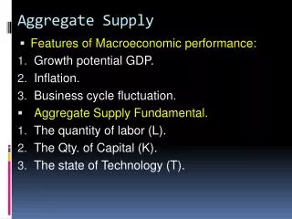
Aggregate Supply Curve Aggregate Supply is the amount of real GDP that will be made available by sellers at various price levels. Aggregate Supply looks different in the Long Run and the Short Run: In the Long Run, classical economists assume the economy operates at full employment (maximum output), independent of the price level. In the Short Run, businesses will increase supply if the price level increases.
Positive Relationship • There is a positive relationship in the short run between price level and the quantity of aggregate output supplied.
The Aggregate Supply Curves The Slope of the Short-Run Aggregate Supply (SAS) Curve • The SAS curve is upward sloping because of: • Auction markets • Prices are determined by demand and supply and supply curves are upward sloping • Posted price markets • Also called quantity-adjusting markets,markets in which firms respond to changes in demand by changing production instead of changing their prices • Firms tend to increase their markup when demand increases
Shifts in the SAS Curve • Shifts in the SAS are caused by changes in: • Input prices • Productivity • Import prices • Excise and sales taxes • When production costs increase, the SAS curve shifts up • In general: • %Δ in price level = • %Δ in wages – %Δ in productivity Price level SAS1 SAS0 SAS2 Real output
The Long-Run Aggregate Supply Curve • The long-run aggregate supply (LAS) curve shows the long-run relationship between output and the price level • The position of the LAS curve depends on potential output which is the amount of goods and services an economy can produce when both capital and labor are fully employed • The LAS curve is vertical because potential output is unaffected by the price level
The LAS Curve Price level LAS • Potential output is assumed to be in the middle of a range bounded by high and low levels of potential output • When resources are over-utilized (point C), factor prices may be bid up and the SAS shifts up SAS Overutilized resources C • When resources are under-utilized (point A), factor prices may decrease and SAS shifts down B Underutilized resources A Real output Low-level potential output High-level potential output
When resources are over-utilized • (point C), factor prices may be bid • up and the SAS shifts up. • When resources are under-utilized • (point A), factor prices may decrease • and SAS shifts down. LAS • Estimating potential output is • inexact, so it is assumed to be the • middle of a range bounded by a • high level of potential output and a • low level of potential output. C • The relationship between • potential and actual output – where • the economy is on SAS – determines • shifts in SAS. B A SAS Price Level Underutilized resources Overutilized resources Real output Low-level potential output High-level potential output • When LAS = SAS (point B), there is • no pressure for prices to rise or fall.
Shifts in the LAS Curve Price level • Increases in the LAS are caused by increases in: • Capital • Resources • Growth-compatible institutions • Technology • Entrepreneurship LAS0 LAS1 LAS2 Real output
LRAS • The long-run aggregate supply curve shows the relationship between the aggregate price level and the quantity of aggregate output supplied that would exist if all prices, including nominal wages, were fully flexible Do you remember the debate between Classical and Keynes?
A Range for Potential Output and the LAS Curve • The position of the long-run aggregate supply curve is determined by potential output. • Potential output – the amount of goods and services an economy can produce when both labor and capital are fully employed. Was this in your textbook?
Short-Run Equilibrium in the AD/AS Model Price level • Short-run equilibrium is where the SAS and AD curves intersect and point E is short-run equilibrium A shift in the aggregate demand curve to the right changes equilibrium from E to F, increasing output from Y0 to Y1 and increasing price level from P0 to P1 SAS P1 P0 F AD1 E AD0 Real output Y0 Y1
Short-Run Equilibrium in the AD/AS Model Price level A shift up in the short-run aggregate supply curve changes equilibrium from E to G, decreasing output from Y0 to Y2 and increasing price level from P0 to P2 SAS1 P2 SAS0 P0 G E AD Real output Y2 Y0
Long-Run Equilibrium in the AD/AS Model • Long-run equilibrium is where the LAS and AD curves intersect Price level LAS A shift in the aggregate demand curve changes equilibrium from E to H, increasing the price level from P0 to P1 but leaving output unchanged H P1 E P0 AD1 AD0 Real output YP
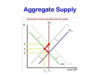
Application:A Recessionary Gap in the AD/AS Model Price level • A recessionary gap is the amount by which equilibrium output is below potential output SAS1 LAS • At point A, some resources are unemployed and the recessionary gap is YP – Y1 SAS0 A P1 Eventually wages and prices decrease and SAS shifts down to return the economy to a long and short-run equilibrium at E E P0 Gap AD0 Real output Y1 YP
Application: An Inflationary Gap in the AD/AS Model Price level • An inflationary gap is the amount by which equilibrium output is above potential output LAS • At point B, resources are being used beyond their potential and the inflationary gap is Y2 – YP SAS0 E P0 SAS2 B Eventually wages and prices increase and SAS shifts to return the economy to a long and short-run equilibrium at E P2 Gap AD0 Real output Y2 YP
From the Short Run to the Long Run Leftward Shift of the Short-run Aggregate Supply Curve
From the Short Run to the Long Run Rightward Shift of the Short-run Aggregate Supply Curve
Aggregate Demand Policy • A primary reason for government policy makers’ interest in the AS/AD model is that monetary or fiscal policy shifts the AD curve • Monetary policy involves the Federal Reserve Bank changing the money supply and interest rates • Fiscal policy is the deliberate change in either government spending or taxes to stimulate or slow down the economy
Application: Expansionary Fiscal Policy in the AD/AS Model Price level • If the economy is at point A, there is a recessionary gap equal to YP – Y0 LAS • The appropriate fiscal policy is to increase government spending and/or decrease taxes P1 E A P0 AD shifts to the right and output returns to potential output YP and prices increase to P1 AD1 Gap AD0 Y0 YP Real output
Application: Contractionary Fiscal Policy in the AD/AS Model Price level • If the economy is point B, there is an inflationary gap Y2 – YP LAS • The appropriate fiscal policy is to decrease government spending and/or increase taxes B P2 P1 AD shifts to the left, output returns to potential output YP and inflation is prevented E AD0 Gap AD2 YP Y2 Real output
Limitations of the AS/AD Model • The AS/AD model assumes away many possible feedback effects that can significantly affect the macroeconomy and lead to quite different conclusions • Implementing fiscal policy through changing taxes and government spending is a slow legislative process • There is no guarantee that government will do what economists say is necessary
Limitations of the AS/AD Model • Potential output (the level of output that the economy is capable of producing without generating inflation) is difficult to estimate • We do have ways to get a rough idea of where it is • There are many other possible interrelationships in the economy that the model does not take into account • The aggregate economy can become dynamically unstable, so a shock can set in motion changes that will not automatically be self-correcting
Limitations of the AS/AD Model • There are two ways to think about the effectiveness of fiscal policy: in the model and in reality • The effectiveness of fiscal policy depends on the government’s ability to perceive and to react appropriately to a problem • Countercyclical fiscal policy is fiscal policy in which the government offsets any change in aggregate expenditures that would create a business cycle • Fine-tuningis used to describe such fiscal policy designed to keep the economy always at its target or potential level of income
Chapter Summary • The key idea of the Keynesian AS/AD model is that in the short run the economy can deviate from potential output • The AS/AD model consists of the aggregate demand curve, and the short-run aggregate supply curve, and the long-run aggregate supply curve • Short-run equilibrium is where the SAS and AD curves intersect; Long-run equilibrium is where the AD and LAS curves intersect • Aggregate demand management policy attempts to influence the level of output in the economy
Chapter Summary • Fiscal policy works by providing a deliberate countershock to offset unexpected shocks to the economy • Macroeconomic policy is difficult to conduct because: • Implementing fiscal policy is a slow process • We don’t really know where potential output is • There are interrelationships not included in the model • The economy can become dynamically unstable