Download
1 / 57
570 likes | 603 Views
Explore a comprehensive overview of direct and iterative solvers for non-symmetric, positive definite matrices, focusing on their robustness, efficiency, and minimal storage requirements. The landscape of sparse Ax=b solvers, including Cholesky factorization, elimination trees, and computational complexities, is analyzed for a deeper understanding of linear solvers. Learn about the time and space complexities involved in solving model problems like Poisson's equation on regular meshes, and the advantages of direct methods over iterative approaches on well-shaped finite element meshes.

E N D
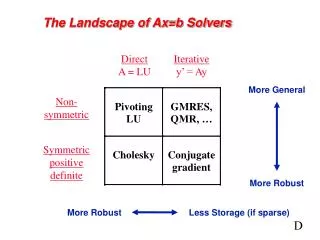
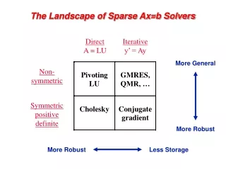
Direct A = LU Iterative y’ = Ay More General Non- symmetric Symmetric positive definite More Robust More Robust Less Storage The Landscape of Sparse Ax=b Solvers
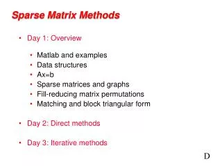
n1/2 n1/3 Complexity of linear solvers Time to solve model problem (Poisson’s equation) on regular mesh
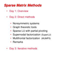
n1/2 n1/3 Complexity of direct methods Time and space to solve any problem on any well-shaped finite element mesh
Sparse Cholesky factorization: A=RTR • Preorder • Independent of numerics • Symbolic Factorization • Elimination tree • Nonzero counts • Supernodes • Nonzero structure of R • Numeric Factorization • Static data structure • Supernodes use BLAS3 to reduce memory traffic • Triangular Solves
for j = 1 : n for k = 1 : j-1 % cmod(j,k) for i = j : n A(i,j) = A(i,j) – A(i,k)*A(j,k); end; end; % cdiv(j) A(j,j) = sqrt(A(j,j)); for i = j+1 : n A(i,j) = A(i,j) / A(j,j); end; end; j LT L A L Column Cholesky Factorization • Column j of A becomes column j of L
for j = 1 : n for k < j with A(j,k) nonzero % sparse cmod(j,k) A(j:n, j) = A(j:n, j) – A(j:n, k)*A(j, k); end; % sparse cdiv(j) A(j,j) = sqrt(A(j,j)); A(j+1:n, j) = A(j+1:n, j) / A(j,j); end; j LT L A L Sparse Column Cholesky Factorization • Column j of A becomes column j of L
Data structures • Full: • 2-dimensional array of real or complex numbers • (nrows*ncols) memory • Sparse: • compressed column storage • about (1.5*nzs + .5*ncols) memory D
3 7 1 3 7 1 6 8 6 8 4 10 4 10 9 2 9 2 5 5 Graphs and Sparse Matrices: Cholesky factorization Fill:new nonzeros in factor Symmetric Gaussian elimination: for j = 1 to n add edges between j’s higher-numbered neighbors G+(A)[chordal] G(A)
3 7 1 6 8 10 4 10 9 5 4 8 9 2 2 5 7 3 6 1 Elimination Tree G+(A) T(A) Cholesky factor • T(A) : parent(j) = min { i > j : (i,j) inG+(A) } • T describes dependencies among columns of factor • Can compute T from G(A) in almost linear time • Can compute G+(A) easily from T D
(Demos in Matlab) • matrix and graph • elimination tree
} O(#nonzeros in A), almost Sparse Cholesky factorization: A=RTR • Preorder • Independent of numerics • Symbolic Factorization • Elimination tree • Nonzero counts • Supernodes • Nonzero structure of R • Numeric Factorization • Static data structure • Supernodes use BLAS3 to reduce memory traffic • Triangular Solves O(#nonzeros in R) O(#flops)
(Demos in Matlab) • orderings in detail
Fill-reducing matrix permutations • Minimum degree: • Eliminate row/col with fewest nzs, add fill, repeat • Theory: can be suboptimal even on 2D model problem • Practice: often wins for medium-sized problems • Nested dissection: • Find a separator, number it last, proceed recursively • Theory: approx optimal separators => approx optimal fill and flop count • Practice: often wins for very large problems • Banded orderings (Reverse Cuthill-McKee, Sloan, . . .): • Try to keep all nonzeros close to the diagonal • Theory, practice: often wins for “long, thin” problems • Best modern general-purpose orderings are ND/MD hybrids.
Fill-reducing permutations in Matlab • Nonsymmetric approximate minimum degree: • p = colamd(A); • column permutation: lu(A(:,p)) often sparser than lu(A) • also for QR factorization • Symmetric approximate minimum degree: • p = symamd(A); • symmetric permutation: chol(A(p,p)) often sparser than chol(A) • Reverse Cuthill-McKee • p = symrcm(A); • A(p,p) often has smaller bandwidth than A • similar to Sparspak RCM D
{ Symmetric Supernodes [Ashcraft, Grimes, Lewis, Peyton, Simon] • Supernode-column update: k sparse vector ops become 1 dense triangular solve + 1 dense matrix * vector + 1 sparse vector add • Sparse BLAS 1 => Dense BLAS 2 • Supernode = group of (contiguous) factor columns with nested structures • Related to clique structureof filled graph G+(A)
G(A) 1 2 3 4 5 6 7 8 9 1 2 3 4 5 6 9 T(A) 7 4 1 7 8 8 9 7 6 3 8 A 6 3 2 5 4 1 2 5 9 Symmetric-pattern multifrontal factorization
G(A) 9 T(A) 4 1 7 8 7 6 3 8 6 3 2 5 4 1 2 5 9 Symmetric-pattern multifrontal factorization For each node of T from leaves to root: • Sum own row/col of A with children’s Update matrices into Frontal matrix • Eliminate current variable from Frontal matrix, to get Update matrix • Pass Update matrix to parent
1 3 7 1 G(A) 3 7 F1 = A1 => U1 9 4 1 7 T(A) 8 3 7 6 3 7 3 8 7 6 3 2 5 4 1 9 2 5 Symmetric-pattern multifrontal factorization For each node of T from leaves to root: • Sum own row/col of A with children’s Update matrices into Frontal matrix • Eliminate current variable from Frontal matrix, to get Update matrix • Pass Update matrix to parent
1 3 7 1 G(A) 3 7 F1 = A1 => U1 9 4 1 7 2 3 9 T(A) 3 9 8 3 7 2 3 6 3 7 3 8 3 9 7 6 3 9 2 5 4 1 9 2 5 F2 = A2 => U2 Symmetric-pattern multifrontal factorization For each node of T from leaves to root: • Sum own row/col of A with children’s Update matrices into Frontal matrix • Eliminate current variable from Frontal matrix, to get Update matrix • Pass Update matrix to parent
1 3 7 1 G(A) 3 7 F1 = A1 => U1 2 3 9 2 3 9 9 4 1 F2 = A2 => U2 7 8 3 3 9 7 3 7 8 9 6 3 7 3 3 3 8 7 8 9 9 7 6 7 3 7 2 5 8 4 1 9 2 5 8 9 9 F3 = A3+U1+U2 => U3 Symmetric-pattern multifrontal factorization T(A)
G(A) 9 T(A) 4 1 7 8 7 6 3 8 6 3 2 5 4 1 2 5 9 Symmetric-pattern multifrontal factorization • Really uses supernodes, not nodes • All arithmetic happens on dense square matrices. • Needs extra memory for a stack of pending update matrices • Potential parallelism: • between independent tree branches • parallel dense ops on frontal matrix
MUMPS: distributed-memory multifrontal[Amestoy, Duff, L’Excellent, Koster, Tuma] • Symmetric-pattern multifrontal factorization • Parallelism both from tree and by sharing dense ops • Dynamic scheduling of dense op sharing • Symmetric preordering • For nonsymmetric matrices: • optional weighted matching for heavy diagonal • expand nonzero pattern to be symmetric • numerical pivoting only within supernodes if possible (doesn’t change pattern) • failed pivots are passed up the tree in the update matrix
(Demos in Matlab) • nonsymmetric LU • dmperm, dmspy, components
Matching and block triangular form • Dulmage-Mendelsohn decomposition: • Bipartite matching followed by strongly connected components • Square, full rank A: • [p, q, r] = dmperm(A); • A(p,q) has nonzero diagonal and is in block upper triangular form • also, strongly connected components of a directed graph • also, connected components of an undirected graph • Arbitrary A: • [p, q, r, s] = dmperm(A); • maximum-size matching in a bipartite graph • minimum-size vertex cover in a bipartite graph • decomposition into strong Hall blocks
GEPP: Gaussian elimination w/ partial pivoting • PA = LU • Sparse, nonsymmetric A • Columns may be preordered for sparsity • Rows permuted by partial pivoting (maybe) • High-performance machines with memory hierarchy P = x
3 7 1 3 7 1 6 8 6 8 4 10 4 10 9 2 9 2 5 5 Symmetric Positive Definite: A=RTR[Parter, Rose] symmetric for j = 1 to n add edges between j’s higher-numbered neighbors fill = # edges in G+ G+(A)[chordal] G(A)
} O(#nonzeros in A), almost Symmetric Positive Definite: A=RTR • Preorder • Independent of numerics • Symbolic Factorization • Elimination tree • Nonzero counts • Supernodes • Nonzero structure of R • Numeric Factorization • Static data structure • Supernodes use BLAS3 to reduce memory traffic • Triangular Solves O(#nonzeros in R) O(#flops)
Modular Left-looking LU Alternatives: • Right-looking Markowitz [Duff, Reid, . . .] • Unsymmetric multifrontal[Davis, . . .] • Symmetric-pattern methods[Amestoy, Duff, . . .] Complications: • Pivoting => Interleave symbolic and numeric phases • Preorder Columns • Symbolic Analysis • Numeric and Symbolic Factorization • Triangular Solves • Lack of symmetry => Lots of issues . . .
Symmetric A implies G+(A) is chordal, with lots of structure and elegant theory For unsymmetric A, things are not as nice • No known way to compute G+(A) faster than Gaussian elimination • No fast way to recognize perfect elimination graphs • No theory of approximately optimal orderings • Directed analogs of elimination tree: Smaller graphs that preserve path structure [Eisenstat, G, Kleitman, Liu, Rose, Tarjan]
2 1 4 5 7 6 3 Directed Graph • A is square, unsymmetric, nonzero diagonal • Edges from rows to columns • Symmetric permutations PAPT A G(A)
2 1 4 5 7 6 3 + L+U Symbolic Gaussian Elimination [Rose, Tarjan] • Add fill edge a -> b if there is a path from a to b through lower-numbered vertices. A G (A)
2 1 4 5 7 6 3 Structure Prediction for Sparse Solve • Given the nonzero structure of b, what is the structure of x? = G(A) A x b • Vertices of G(A) from which there is a path to a vertex of b.
1 2 3 4 5 = 1 3 5 2 4 Sparse Triangular Solve L x b G(LT) • Symbolic: • Predict structure of x by depth-first search from nonzeros of b • Numeric: • Compute values of x in topological order Time = O(flops)
for column j = 1 to n do solve pivot: swap ujj and an elt of lj scale:lj = lj / ujj j U L A ( ) L 0L I ( ) ujlj L = aj for uj, lj Left-looking Column LU Factorization • Column j of A becomes column j of L and U
GP Algorithm [G, Peierls; Matlab 4] • Left-looking column-by-column factorization • Depth-first search to predict structure of each column +: Symbolic cost proportional to flops -: BLAS-1 speed, poor cache reuse -: Symbolic computation still expensive => Prune symbolic representation
j k r r = fill Symmetric pruning:Set Lsr=0 if LjrUrj 0 Justification:Ask will still fill in j = pruned = nonzero s Symmetric Pruning [Eisenstat, Liu] Idea: Depth-first search in a sparser graph with the same path structure • Use (just-finished) column j of L to prune earlier columns • No column is pruned more than once • The pruned graph is the elimination tree if A is symmetric
GP-Mod Algorithm [Matlab 5-6] • Left-looking column-by-column factorization • Depth-first search to predict structure of each column • Symmetric pruning to reduce symbolic cost +: Symbolic factorization time much less than arithmetic -: BLAS-1 speed, poor cache reuse => Supernodes
{ Symmetric Supernodes [Ashcraft, Grimes, Lewis, Peyton, Simon] • Supernode-column update: k sparse vector ops become 1 dense triangular solve + 1 dense matrix * vector + 1 sparse vector add • Sparse BLAS 1 => Dense BLAS 2 • Supernode = group of (contiguous) factor columns with nested structures • Related to clique structureof filled graph G+(A)
1 1 2 2 3 3 4 4 5 5 6 6 7 7 8 8 9 9 10 10 Factors L+U Nonsymmetric Supernodes Original matrix A
for each panel do Symbolic factorization:which supernodes update the panel; Supernode-panel update:for each updating supernode do for each panel column dosupernode-column update; Factorization within panel:use supernode-column algorithm +: “BLAS-2.5” replaces BLAS-1 -: Very big supernodes don’t fit in cache => 2D blocking of supernode-column updates j j+w-1 } } supernode panel Supernode-Panel Updates
Sequential SuperLU [Demmel, Eisenstat, G, Li, Liu] • Depth-first search, symmetric pruning • Supernode-panel updates • 1D or 2D blocking chosen per supernode • Blocking parameters can be tuned to cache architecture • Condition estimation, iterative refinement, componentwise error bounds
SuperLU: Relative Performance • Speedup over GP column-column • 22 matrices: Order 765 to 76480; GP factor time 0.4 sec to 1.7 hr • SGI R8000 (1995)
1 2 3 4 5 3 1 2 3 4 5 1 4 5 2 3 4 5 2 1 Column Intersection Graph • G(A) = G(ATA) if no cancellation(otherwise) • Permuting the rows of A does not change G(A) A ATA G(A)
1 2 3 4 5 3 + 1 2 3 4 5 G(A) 1 4 5 2 3 4 2 5 1 + + + Filled Column Intersection Graph • G(A) = symbolic Cholesky factor of ATA • In PA=LU, G(U) G(A) and G(L) G(A) • Tighter bound on L from symbolic QR • Bounds are best possible if A is strong Hall [George, G, Ng, Peyton] A chol(ATA)
5 1 2 3 4 5 1 2 3 4 5 1 4 2 2 3 3 4 5 1 Column Elimination Tree • Elimination tree of ATA (if no cancellation) • Depth-first spanning tree of G(A) • Represents column dependencies in various factorizations T(A) A chol(ATA) +
k j T[k] • If A is strong Hall then, for some pivot sequence, every column modifies its parent in T(A). [G, Grigori] Column Dependencies in PA = LU • If column j modifies column k, then j T[k]. [George, Liu, Ng]
Efficient Structure Prediction Given the structure of (unsymmetric) A, one can find . . . • column elimination tree T(A) • row and column counts for G(A) • supernodes of G(A) • nonzero structure of G(A) . . . without forming G(A) or ATA [G, Li, Liu, Ng, Peyton; Matlab] + + +
Shared Memory SuperLU-MT [Demmel, G, Li] • 1D data layout across processors • Dynamic assignment of panel tasks to processors • Task tree follows column elimination tree • Two sources of parallelism: • Independent subtrees • Pipelining dependent panel tasks • Single processor “BLAS 2.5” SuperLU kernel • Good speedup for 8-16 processors • Scalability limited by 1D data layout
SuperLU-MT Performance Highlight (1999) 3-D flow calculation (matrix EX11, order 16614):
= x Column Preordering for Sparsity Q • PAQT= LU:Q preorders columns for sparsity, P is row pivoting • Column permutation of A Symmetric permutation of ATA (or G(A)) • Symmetric ordering: Approximate minimum degree [Amestoy, Davis, Duff] • But, forming ATA is expensive (sometimes bigger than L+U). • Solution: ColAMD: ordering ATA with data structures based on A P


![SAT and CSP/CP Solvers [complete search]](https://cdn1.slideserve.com/2014486/slide1-dt.jpg)