Download

1 / 40
400 likes | 547 Views
Basics of mm interferometry. Sébastien Muller Nordic ARC Onsala Space Observatory, Sweden. Turku Summer School – June 2009. Interests of mm radioastronomy. -> Cold Universe Giant Molecular Clouds -> COLD and DENSE phase Site of the STAR FORMATION -> Continuum emission of cold dust

E N D
Basics of mm interferometry Sébastien Muller Nordic ARC Onsala Space Observatory, Sweden Turku Summer School – June 2009
Interests of mm radioastronomy -> Cold Universe Giant Molecular Clouds -> COLD and DENSE phase Site of the STAR FORMATION -> Continuum emission of cold dust -> Molecular transitions - Diagnostics of the gas properties (temperature, density) - Kinematics (outflows, rotation)
Where the atmosphere is relatively transparent Interests of CO Molecular gas H2 But H2 symmetric ->electric dipolar momentum is 0 Most abundant molecule after H2 is CO [CO/H2] ~ 10-4 First rotational transitions of CO in the mm CO(1-0) @115 GHz CO(2-1) @230 GHz CO(3-2) @345 GHz E J=1,2,3 = 6, 17, 33 K Easily excited CO is difficult to destroy high ionization potential (14eV) and dissociation energy (11 eV)
Handy formulae - HI line emission: N(HI) (cm-2) = 1.82 1018TBdv (K km/s) - Molecular line emission: N(H2) (cm-2) = X 1020TCOdv (K km/s) X = 0.5-3 Or use optically thin lines (13CO, C18O) - Visual extinction: N(HI)+2N (H2) (cm-2) = 2 1021AV (mag)
Needs of angular resolution Resolution /D (theory of diffraction)
Would need very large single-dish antennas BUT - Surface accuracy(few 10s of microns !) -> technically difficult and expensive ! - Small field of view (1 pixel) - Pointing accuracy (fraction of the beam) Let’s fill in a large collecting area with small antennas And combine the signal they receive -> Interferometry (Aperture synthesis)
Mm antennas need Good surface accuracy D APEX 12m <20 microns IRAM-30m 30m 55 microns (GBT 100m 300 microns) PdBI 15m <50 microns SMA 6m <20 microns ALMA 12m <25 microns
source uv plane geometrical time delay antenna baseline Baseline, uv plane and spatial frequency • uv positions are the projection of the baseline vectors • Bij as seen from the source. • The distances (u2 + v2) are refered to as spatial frequencies • Interferometers can access the spatial frequencies • ONLY between Bmin and Bmax, the shortest and longest • projected baselines respectively.
Interferometers measure VISIBILITIES V V(u,v) = P(x,y) I(x,y) exp –i2(ux+vy) dxdy = FT{ P I } But astronomers want the SKY BRIGHTNESS DISTRIBUTION of the source : I(x,y) P(x,y) is the PRIMARY BEAM of the antennas - P has a finite support, so the field of view is limited - distorded source informations - P is in principle known ie. antenna characteristic
I(x,y) P(x,y) = V(u,v) exp i2(ux+vy) dudv Well, looks easy … BUT ! Interferometers have an irregular and limited uv sampling : - high spatial frequency (limit the resolution) - low spatial frequency (problem with wide field imaging) Incomplete sampling, non respect of the Nyquist’s criterion = LOSS of informations ! The direct deconvolution is not possible Need to use some smart algorithms (e.g. CLEAN)
I x x0 Phase Amplitude S Slope = -2x0 u u Let’s take an easy example: 1D P = 1 I(x) = Dirac function: S(x-x0) S = constant V(u) = FT(I) = Sexp(-i2ux0) -> this is a complex value
Illustration : dirty beam, dirty image and deconvolved (clean) image resulting in some interferometric observations of a source model
Atmosphere « The atmosphere is the worst part of an astronomical instrument » - emits thermally, thus add noise - absorbs incoming radiation - is turbulent ! (seeing) Changes in refractive index introduce phase delay Phase noise -> DECORRELATION(more on long baselines) exp(-2/2) - Main enemy is water vapor (Scale height ~2 km)
O2 H2O
Calibration Vobs = G Vtrue + N Vobs = observed visibilities Vtrue = true visibilies = FT(sky) G = (complex) gains usually can be decomposed into antenna-based terms: G = Gij= Gi x Gj* N = noise After calibration: Vcorr = G’ –1 Vobs
Calibration - Frequency-dependent response of the system Bandpass calibration -> Bright continuum source - Time-dependent response of the system Gain (phase and amplitude) -> Nearby quasars - Absolute flux scale calibration -> Flux calibrator
From SMA Observer Center Tools http://sma1.sma.hawaii.edu/
From SMA Observer Center Tools http://sma1.sma.hawaii.edu/
From SMA Observer Center Tools http://sma1.sma.hawaii.edu/
Quasars usually variable ! -> need reliable flux calibrator From SMA Observer Center Tools http://sma1.sma.hawaii.edu/
Preparing a proposal 0) Search in Archives SMA: http://www.cfa.harvard.edu/cgi-bin/sma/smaarch.pl PdBI: http://vizier.cfa.harvard.edu/viz-bin/VizieR?-source=B/iram ALMA … 1) Science justifications -> Model(s) to interpret the data 2) Technical feasibility: - Array configuration(s) (angular resolution, goals) - Sensitivity use Time Estimator ! Point source sensitivity Brightness sensitivity (extended sources)
Array configuration Compact Detection Mapping of extended regions Intermediate Mapping Extended High angular resolution mapping Astrometry Very-extended Size measurements Astrometry
PdBI 1 Jy = 10-26 W m-2 Hz-1
For extended source: Take into account the synthesized beam -> brightness sensitivity T (K) = 2ln2c2/k2 x Flux density/majmin Use Time Estimator !
Short spacings V(u,v) = P(x,y) I(x,y) exp –i2(ux+vy) dxdy V(0,0) = P(x,y) I(x,y) dxdy (Forget P), this is the total flux of the source And it is NOT measured by an interferometer ! -> Problem for extended sources !!! -> Try to fill in the short spacings
Advantages of interferometers - High angular resolution - Large collecting area - Flatter baselines - Astrometry - Can filter out extended emission - Large field of view with independent pixels - Flexible angular resolution (different configuration)
Disadvantages of interferometers - Require stable atmosphere - High altitude and ~flat site (usually difficult to access) - Lots of receivers to do - Complex correlator - Can filter out extended emission - Need time and different configuration to fill in the uv-plane
Mm interferometry: summary - Essential to study the Cold Universe (SF) - Astrophysics: temperature, density, kinematics … - Robust technique High angular resolution High spectral/velocity resolution
Let’s define - Sampling function S(u,v) = 1 at (u,v) points where visibilities are measured = 0 elsewhere - Weighting function W(u,v) = weights of the visibilities (arbitrary) We get : Iobs(x,y) = V(u,v) S(u,v) W(u,v) exp i2(ux+vy) dudv
Due to the Fourier Transform properties : FT { A B } = FT { A } ** FT { B } Can be rewritten as : where Iobs(x,y) = V(u,v) S(u,v) W(u,v) exp i2(ux+vy) dudv Iobs(x,y) = P(x,y) I(x,y) ** D(x,y) D(x,y) = S(u,v) W(u,v) exp i2(ux+vy) dudv = FT { S W }
Iobs(x,y) = P(x,y) I(x,y) ** D(x,y) If Isou = (x,y) = Point source then Iobs(x,y) = D(x,y) That is : D is the image of a point source as seen by the interferometer. ~ Point Spread Function
D(x,y) = FT { S W } D(x,y) is called DIRTY BEAM This dirty beam depends on : - the uv sampling (uv coverage) S - the weighting function W Note that : D(x,y) dxdy = 0 because S(0,0) = 0 And that : D(0,0) > 0 because SW > 0 The dirty beam presents a positive peak at the center, surrounded by a complex pattern of positive and negative sidelobes, which depends on the uv coverage and the weighting function.
Iobs(x,y) = P(x,y) I(x,y) ** D(x,y) Iobs(x,y) is called DIRTY IMAGE We want Iobs(x,y) I(x,y) This includes the two key issues for imaging : - Fourier Transform (to obtain Iobs from V and S) - Deconvolution (to obtain I from Iobs)