Laboratory in Oceanography: Data and Methods Observations vs. Models

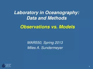
1. Laboratory in Oceanography: Data and Methods Observations vs. Models MAR550, Spring 2013 Miles A. Sundermeyer

2. Observations vs. Models • Observational data • Numerous steps involved in making and interpreting observations: • turn environmental signal to something we can measure (e.g., resistance or voltage in case of thermister) • signal conditioning – e.g., operational amplifier, low pass filter • discrete sampling – e.g., A/D converter, determines sampling rate/frequency, resolution/precision • internal processing - e.g., conditional sampling, averaging, etc. • data storage • calibration • processing/analysis

3. Observations vs. Models • Observational data • The ocean is a fundamentally a continuous environment • When we sample it, we make a finite number of discrete measurements • When we make discrete measurements, we also: • subsample • average

4. Observations vs. Models

5. Observations vs. Models

6. Observations vs. Models

7. Observations vs. Models

8. Observations vs. Models

9. Observations vs. Models

10. Observations vs. Models

11. Observations vs. Models • Measured vs. computed variables • Some of the quantities we observe are properties of the water, others are environmental variables, • e.g., salinity is a property of water, velocity is an environmental variable • Some quantities we wish to observe are directly measured, some are computed from measured quantities; • e.g., temperature is measured (sort of), salinity is computed • Measurement noise / uncertainty • Observations can contain noise from either: • Instrument noise / sampling error • Environmental variability at unresolved / unknown scales

12. Observations vs. Models • Instrument calibration • Once observations are made, sensor output converted / interpreted to yield physical units of variable being measured • e.g., CTD returns voltages, which are converted to conductivity and temperature, which are used to compute salinity

13. Observations vs. Models Other considerations for observational data accuracy - how well the sensor measures the environment in an absolute sense resolution / precision - the ability of a sensor to see small differences in readings e.g. a temperature sensor may have a resolution of 0.000,01º C, but only be accurate to 0.001º C range - the maximum and minimum value range over which a sensor works well. repeatability - ability of a sensor to repeat a measurement when put back in the same environment - often directly related to accuracy drift/stability - low frequency change in a sensor with time - often associated with electronic aging of components or reference standards in the sensor hysteresis - present state depends on previous state; e.g., a linear up and down input to a sensor, results in output that lags the input, i.e., one curve on increasing pressure, and another on decreasing response time - typically estimated as the frequency response of a sensor assuming exponential behavior self heating - to measure the resistance in the thermistor to measure temperature, we need to put current through it settling time - the time for the sensor to reach a stable output once it is turned on

14. Observations vs. Models • How do we define a “model?” • Theoretical model - an abstraction or conceptual object used in the creation of a predictive formula • Computer model - a computer program which attempts to simulate an abstract model of a particular system • Laboratory model - a laboratory apparatus that reproduces a particular observed dynamic / characteristic • Mathematical model - an abstract model that uses mathematical language • Statistical model - in applied statistics, a parameterized set of probability distributions

15. Observations vs. Models Example: Analytical model Equations of motion – e.g., Boussinesq equations and advection / diffusion equation for passive tracer

16. Observations vs. Models Example: Numerical model

17. Observations vs. Models • Numerical model data • For numerical models, effectively replace first two steps with: • continuous equations representing problem to be solved, e.g, Navier-Stokes equations. • reduce the equations to simplified form appropriate to problem of interest • discretized version of these in form of numerical model (finite difference, volume, Fourier modes, etc.) • ... • signal conditioning – e.g., operational amplifier, low pass filter • discrete sampling – e.g., A/D converter, determines sampling rate/frequency, resolution/precision • internal processing - e.g., conditional sampling, averaging, etc. • data storage • calibration • processing/analysis

18. Observations vs. Models Example: Statistical model

19. Observations vs. Models Example: Laboratory model Vertically oscillated grid mixers Top View

20. Observations vs. Models Example: Regression / curve fitting to data yi = mxi + b y = Xb

21. Observations vs. Models • Purpose of Models • Wish to be able to predict/describe the state of the ocean environment based on some form of model • Need to be able to go from one type of model to another to better understand each – sometimes models seem as complicated as real world • Ultimately seek to understand the ocean environment • Interpret observations with the context of models • Formulate new models based on observations

22. Total Flowrate 300 Salinity Concentration Neap 32.0 250 Spring Neap Spring 30.0 200 150 28.0 SAL (ppt) /sec) Flowrate (ft 100 26.0 3 50 24.0 0 -50 22.0 -100 20.0 -500 -400 -300 -200 -100 0 100 200 300 400 500 600 -150 Time (minutes since High Tide) -200 -500 -400 -300 -200 -100 0 100 200 300 400 500 600 Time (minutes since High Tide) Observations vs. Models Example: Allens Pond, Westport, MA Data and figures courtesy of Case Studies in Estuarine Dynamics (MAR620) project team, Spring 2008

23. Observations vs. Models Example: Allens Pond, Westport, MA (cont’d) • Conceptual Model of Allens Pond: • Estuary connected to ocean via frictional sill • Tidal range in open water extends below sill. High water mark Outer Stage

24. Observations vs. Models Example: Allens Pond, Westport, MA (cont’d) • Theoretical Model of Allens Pond: • Frictional flow, i.e., pressure gradient balanced by friction • Assume hydrostatic balance: • Assume quadratic drag law: • Volume conservation:

25. Observations vs. Models Example: Allens Pond, Westport, MA (cont’d) Total Flowrate 300 Neap 250 Spring 200 150 /sec) Flowrate (ft 100 3 50 0 -50 -100 -150 -200 -500 -400 -300 -200 -100 0 100 200 300 400 500 600 Time (minutes since High Tide)