Download
1 / 17
190 likes | 453 Views
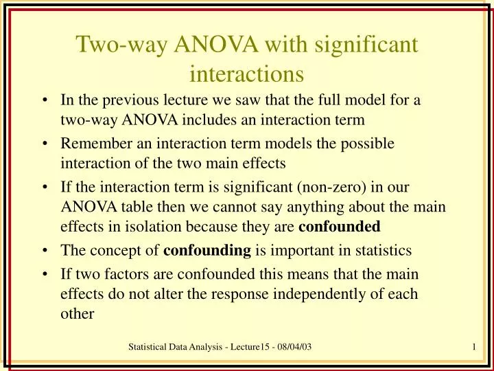
Two-way ANOVA with significant interactions. In the previous lecture we saw that the full model for a two-way ANOVA includes an interaction term Remember an interaction term models the possible interaction of the two main effects

E N D
Two-way ANOVA with significant interactions • In the previous lecture we saw that the full model for a two-way ANOVA includes an interaction term • Remember an interaction term models the possible interaction of the two main effects • If the interaction term is significant (non-zero) in our ANOVA table then we cannot say anything about the main effects in isolation because they are confounded • The concept of confounding is important in statistics • If two factors are confounded this means that the main effects do not alter the response independently of each other Statistical Data Analysis - Lecture15 - 08/04/03
Example • The data on the following slide come from an experiment carried out by a statistics class • They planted 100 seeds in each of 48 boxes and applied two treatments • The boxes were left uncovered or covered • The students watered the seed boxes each day with a preset amount of water (coded levels 1 through 6) • So the 48 boxes were divided into 24 left uncovered and 24 left covered. The watering levels were assigned in equal proportions, so 4 boxes out of 24 receive level 1, 4 receive level 2 and so on • Therefore the design is balanced (equal numbers of replicates for each treatment combination) • At the end of two weeks the students counted how many seeds had germinated in each box Statistical Data Analysis - Lecture15 - 08/04/03
Example • In this experiment: • The number of seeds that germinated is our response • LIGHT and WATER are our two factors • The factor LIGHT has two levels (uncovered/covered) • The factor WATER has six levels corresponding to the amount of water given • Therefore our probability model is In words we say that “the number of seeds that germinate is dependent on whether the box is covered or not and the amount of water the box receives plus some effect due to the interaction of these two factors. We expect the residuals in this model to be Normally distributed with mean zero and variance sigma squared” Statistical Data Analysis - Lecture15 - 08/04/03
What do we know? • What do we know before we carry out this experiment? • Plants need light to live (to carry out photosynthesis) • Plants need water to live • Plants do not survive (well) on water alone • Plants do not survive at all on light alone • Too much water is not good for plants that don’t live in the water • Therefore, we expect that there will be an interaction between the factors LIGHT and WATER Statistical Data Analysis - Lecture15 - 08/04/03
Two way interaction with ANOVA Statistical Data Analysis - Lecture15 - 08/04/03
is an integer, where Two-way ANOVA with missing values • From the table on the previous slide we can see that the experimenters did not get a result from the 4th uncovered replicate with watering level 5 • Some statistical packages have a little trouble with missing values or unbalanced designs. Minitab does. R does not. • In general an experiment with two factors with levels I and J respectively is balanced if Statistical Data Analysis - Lecture15 - 08/04/03
Two-way ANOVA in R • Read in the data seeds<-read.csv(“seeds.csv”) • Make sure the factors are coded as factors seeds$Light<-as.factor(seeds$Light) seeds$Water<-as.factor(seeds$Water) • Fit the model fit<-aov(Count~Light*Water,data=seeds) • Check the model plot(fit) • Get the ANOVA table anova(fit) Statistical Data Analysis - Lecture15 - 08/04/03
Analysis of Variance Table Response: Count Df Sum Sq Mean Sq F value Pr(>F) Light 1 3.6 3.6 0.0857 0.7715 Water 5 28995.0 5799.0 136.7303 < 2.2e-16 *** Light:Water 5 6017.8 1203.6 28.3779 2.174e-11 *** Residuals 35 1484.4 42.4 --- • From the ANOVA table we can see that the P-value for the hypothesis test that the interactions are zero is <0.001 • I.e. there is very strong evidence against the null hypothesis that the interactions are zero • This is what we expected to see • However, do the model assumptions hold? • If the responses can range from zero to one hundred (no seeds germinated – all seeds germinated), then this is a clear violation of the assumption of normality • Does it matter? Statistical Data Analysis - Lecture15 - 08/04/03
Normality assumptions • Norplot is approximately linear • Therefore the assumption of Normality whilst not strictly true is at least not violated too badly • The least squares line (regressing residuals on Z-scores) is of y = -1.4E-15 + 5.56997x, or approximately y = 0 + 5.6x = 5.6x • I.e. the residuals are approximately normally distributed with mean 0 and standard deviation 5.6 • Therefore +/- 3sd = +/-16.8 • We have one residual of –17.25 (z-score 3.08) so not too bad Statistical Data Analysis - Lecture15 - 08/04/03
Pred-res plot • The pred-res plot is hard to interpret with only 4 observations per group • We might be concerned about the water level 6 data (all the counts are zero) • What happens when we analyse the experiment without it? • Use the subs parameter in aov, e.g. fit2<-aov(Count~Light*Water,data=seeds ,subs=-((1:48)[Water==6])) • Makes little difference to the ANOVA table or the residual plots Statistical Data Analysis - Lecture15 - 08/04/03
A graphical display of two-way data (interaction plots) • We can construct LSD plots for two-way data • The process is just the same as for one-way, but now we have a mean for each combination of the factor levels, i.e. • E.g. we have 2 levels for light and 6 levels for water, so we have 12 fitted means and standard deviations. The degrees of freedom are now min(nij-1, i=1..I, j=1..J) (3 for our example) • However, it may be more informative to look at a plot of how the means vary with the combinations of the factors Statistical Data Analysis - Lecture15 - 08/04/03
Interaction plots • Interaction plots plot the means for each combination of the levels of the factors • The plot places the levels of one factor on the x-axis and the mean levels of the other factor on the y-axis, i.e • Factors 1 to I on the x-axis • on the y-axis • A point is then plotted for each data mean • It is traditional to join the means with the same j level in the y-axis factor with a line • I.e. join up • If the lines are parallel and not overlapping then there is little or no evidence of an interaction in the data • If the lines overlap or are not parallel, then this is taken as evidence of a significant interaction • For the examples we’re considering it should make no difference whether we use data means or fitted means Statistical Data Analysis - Lecture15 - 08/04/03
Interpretation • We know from our ANOVA table that the interaction is significant • This is represented by the overlapping lines • We can see that the uncovered boxes have more successful germinations with less water than the uncovered boxes • We can see that water level 6 is fatal regardless of light • We can see that light is less important than water (in that we can achieve similar germination levels with more water and no light • It looks like the covered boxes may be more robust to water level Statistical Data Analysis - Lecture15 - 08/04/03