Introduction to Regression Analysis
Introduction to Regression Analysis. Straight lines, fitted values, residual values, sums of squares, relation to the analysis of variance. Population characteristics. Expected value Is a conditional mean: it is dependent on The conditional mean is called the regression

Introduction to Regression Analysis
E N D
Presentation Transcript
Introduction to Regression Analysis Straight lines, fitted values, residual values, sums of squares, relation to the analysis of variance
Population characteristics • Expected value • Is a conditional mean: it is dependent on • The conditional mean is called the regression • When this mean is a straight line, we write
The Errors • Are independent • This assumption is important • Excluded: Longitudinal data; repeated measures; split units; cross overs; clustering
The sample gives the estimates of the population characteristics • For example: • Some books write: • Your choice (but be clear!)
A simple example • X Y • 1 2 • 2 3 • 3 3 • 4 7 • 5 10
Residual Sum of Squares • Without X: • With X: • The difference is the sum of squares ‘attributable’ to X: The Regression SS
Analysis of variance table • Source SS df MS • Regression 40 1 40 • Residual 6 3 2 • Total 46 4 • F = 40/2 = 20 cf F(1,3) • p-value = P(F > 20) = 0.0208
Regression analysis • . regr y x • Source | SS df MS Number of obs = 5 • -------------+------------------------------ F( 1, 3) = 20.00 • Model | 40 1 40 Prob > F = 0.0208 • Residual | 6 3 2 R-squared = 0.8696 • -------------+------------------------------ Adj R-squared = 0.8261 • Total | 46 4 11.5 Root MSE = 1.4142 • ------------------------------------------------------------------------------ • y | Coef. Std. Err. t P>|t| [95% Conf. Interval] • -------------+---------------------------------------------------------------- • x | 2 .4472136 4.47 0.021 .5767667 3.423233 • _cons | -1 1.48324 -0.67 0.548 -5.720331 3.720331 • ------------------------------------------------------------------------------
Centering • . gen xc=x-3 • . regr y xc • Source | SS df MS Number of obs = 5 • -------------+------------------------------ F( 1, 3) = 20.00 • Model | 40 1 40 Prob > F = 0.0208 • Residual | 6 3 2 R-squared = 0.8696 • -------------+------------------------------ Adj R-squared = 0.8261 • Total | 46 4 11.5 Root MSE = 1.4142 • ------------------------------------------------------------------------------ • y | Coef. Std. Err. t P>|t| [95% Conf. Interval] • -------------+---------------------------------------------------------------- • xc | 2 .4472136 4.47 0.021 .5767667 3.423233 • _cons | 5 .6324555 7.91 0.004 2.987244 7.012756 • ------------------------------------------------------------------------------