Download
1 / 26
260 likes | 382 Views
This document presents an in-depth exploration of discriminative n-gram language modeling, focusing on global linear models, particularly the perceptron algorithm and global conditional log-linear models (GCLMs). It outlines key concepts such as the representation of n-gram language models, implementation for speech recognition using weighted finite automata, and the optimization of model parameters. Theoretical underpinnings are supported by theorems ensuring convergence to globally optimal solutions, addressing common issues like over-training, and providing a comprehensive understanding of the algorithms that underpin modern language processing methods.

E N D
Discriminative n-gram language modeling Brian Roark, Murat Saraclar, Michael Collins Presented by Patty Liu
Outline • Global linear models - The perceptron algorithm - Global conditional log-linear models (GCLM) • Linear models for speech recognition - The basic approach - Implementation using WFA - Representation of n-gram language models - The perceptron algorithm - Global conditional log-linear models
Global linear models • The task is to learn a mapping from inputs to outputs . • We assume the following components: (1) Training examples , for . (2) A function which enumerates a finite set of candidates for each possible input . (3) A representation mapping each to a feature vector . (4) A parameter vector .
Global linear models─ The perceptron algorithm(1/2) Inputs: Training examples Initialization: Set Algorithm: For t = 1…T For i = 1…N Calculate If then Output: Parameters Definition 1. Let In other words is the set of incorrect candidates for an example . We will say that a training sequenceis separable with margin if there exists some vector U with such that ||U|| is the 2-norm of U, i.e., .
Global linear models─ The perceptron algorithm(2/2) • : the number of times an error is made by the algorithm, that is, the number of times that the condition is met at any point in the algorithm Theorem 1. For any training sequence that is separable with margin , for any value of T , then for the perceptron algorithm in Fig. 1 Where R is a constant such that
Global linear models ─ GCLM (1/3) • Global conditional log-linear models (GCLMs) use the parameters a to define a conditional distribution over the members of for a given input : where is a normalization constant that depends on and . • The log-likelihood of the training data under parameters is :
Global linear models ─ GCLM (2/3) • We use a zero-mean Gaussian prior on the parameters resulting in the regularized objective function: • The value dictates the relative influence of the log-likelihood term vs. the prior, and is typically estimated using held-out data. • The optimal parameters under this criterion are . • The derivative of the objective function with respect to a parameter at parameter values is:
Global linear models ─ GCLM (3/3) • is a convex function, so that there are no issues with local maxima in the objective function, and the optimization methods we use converge to the globally optimal solution. • The use of the Gaussian prior term effectively ensures that there is a large penalty for parameter values in the model becoming too large – as such, it tends to control over-training.
Linear models for speech recognition─ The basic approach (1/2) • In the language modeling setting we take to be the set of all possible acoustic inputs; is the set of all possible strings, , for some vocabulary . • Each is an utterance (a sequence of acoustic feature-vectors), and is the set of possible transcriptions under a first pass recognizer. ( is a huge set, but will be represented compactly using a lattice) • We take to be the member of with lowest error rate with respect to the reference transcription of . • feature-vector representation:
Linear models for speech recognition─ The basic approach (2/2) • , which is defined as the log-probability of in the lattice produced by the baseline recognizer. • The lattice is deterministic, so that any word sequence has at most one path through the lattice. • Thus multiple time-alignments for the same word sequence are not represented; the path associated with a word sequence is the path that receives the highest probability among all competing time alignments for that word sequence.
Linear models for speech recognition─ Implementation using WFA (1/9) ◎ Definition: For our purpose, a WFA is a tuple . • : the vocabulary • : a (finite) set of states • :a unique start state • :is a set of final states • :a (finite) set of transitions • :a function from final states to final weights
Linear models for speech recognition─ Implementation using WFA (2/9) • Each transition is a tuple - :a label (in our case, a word) - :the origin state of - :the destination state of - :the weight of the transition • A successful path is a sequence of transitions, such that . • Let be the set of successful paths in a WFA . For any .
Linear models for speech recognition─ Implementation using WFA (3/9) • The weights of the WFA in our case are always in the log semiring, which means that the weight of a path is defined as: • All WFA that we will discuss in this paper are deterministic, i.e. there are no transitions, and for any two transitions . • Thus, for any string , there is at most one successful path , such that and for . • The set of strings such that there exists a with define a regular language .
Linear models for speech recognition─ Implementation using WFA (4/9) Definition of some operations : • : - For a set of transitions and , define . - Then, for any WFA , define for as follows: . • : - The intersection of two deterministic WFAs in the log semiring is a deterministic WFA such that . - For any .
Linear models for speech recognition─ Implementation using WFA (5/9) • : This operation takes a WFA , and returns the best scoring path . • : - Given a WFA , a string , and an error-function , this operation returns . - This operation will generally be used with as the reference transcription for a particular training example, and as some measure of the number of errors in when compared to . - In this case, the operation returns the path such has the smallest number of errors when compared to .
Linear models for speech recognition─ Implementation using WFA (6/9) • : - Given a WFA , this operation yields a WFA , such that and for every there is a such that and . - Note that . In other words the weights define a probability distribution over the paths. • : Given a WFA and an n-gram , we define the expected count of in as where is defined to be the number of times the n-gram appears in a string .
Linear models for speech recognition─ Implementation using WFA (7/9) ◎ Decoding: • producing a lattice L from the baseline recognizer • scaling with and intersecting it with the discriminative language model • finding the best scoring path in the new WFA
Linear models for speech recognition─ Implementation using WFA (8/9) ◎ Goal: • : Given an acoustic input , let be a deterministic word-lattice produced by the baseline recognizer. • The lattice is an acyclic WFA, representing a weighted set of possible transcriptions of under the baseline recognizer. • The weights represent the combination of acoustic and language model scores in the original recognizer. • : The new, discriminative language model constructed during training consists of a deterministic WFA.
Linear models for speech recognition─ Implementation using WFA (9/9) ◎ Training: • Given a training set , where is an acoustic sequence, and is a reference transcription, we can construct lattices using the baseline recognizer. • target transcriptions • The training algorithm is then a mapping from to a pair . • The construction of the language model requires two choices: (1) the choice of the set of n-gram features (2) the choice of parameters
Linear models for speech recognition─ Representation of n-gram language models (1/2) • Every state in the automaton represents an n-gram history , e.g. . • There are transitions leaving the state for every word such that the feature has a weight.
Linear models for speech recognition─ Representation of n-gram language models (2/2) • The failure transition points to the back-off state , i.e. the n-gram history minus its initial word. • The entire weight of all features associated with the word following history must be assigned to the transition labeled with leaving the state in the automaton. For example, if , then the trigram is a feature, as is the bigram and the unigram .
Linear models for speech recognition─ The perceptron algorithm • :a best scoring path • :a minimum error path • Experiments suggest that the perceptron reaches optimal performance after a small number of training iterations, for example T = 1 or T = 2. Inputs: Lattices and reference transcriptions A value for the parameter Initialization: Set to be a WFA that accepts all strings in with weight 0. Set Algorithm: For t = 1. . .T, i = 1. . .N: ‧Calculate ‧For all j for j = 1. . .d such that apply the update Modify to incorporate these parameter changes.
Linear models for speech recognition─ GCLM (1/4) • The optimization method requires calculation of and the gradient of for a series of values for . • The first step in calculating these quantities is to take the parameter values , and to construct an acceptor D which accepts all strings in , such that • For each training lattice , we then construct a new lattice . The lattice represents (in the log domain) the distribution over strings . • The value of for any can be computed by simply taking the path weight of such that in the new lattice . Hence computation of is straightforward.
Linear models for speech recognition─ GCLM (2/4) • To calculate the n-gram feature gradients for the GCLM optimization, the quantity below must be computed. • The first term is simply the number of times the th n-gram feature is seen in . • The second term is the expected number of times that the th n-gram is seen in the acceptor . If the th n-gram is , then this can be computed as .
Linear models for speech recognition─ GCLM (3/4) • , the log probability of the path, is decomposed to be the sum of log probabilities of each transition in the path. We index each transition in the lattice , and store its log probability under the baseline model. • We found that an approximation to the gradient of , however, performed nearly identically to this exact gradient, while requiring substantially less computation. - Let be a string of n words, labeling a successful path in word-lattice . - :the conditional probability under the current model
Linear models for speech recognition─ GCLM (4/4) - :the probability of in the normalized baseline ASR lattice - :the set of strings in the language defined by • Then we wish to compute • The approximation is to make the following Markov assumption: - :the set of all trigrams seen in