N-gram model limitations

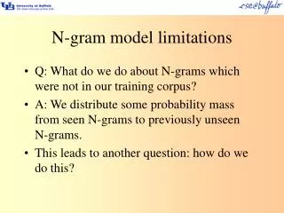
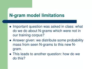
1. N-gram model limitations • Important question was asked in class: what do we do about N-grams which were not in our training corpus? • Answer given: we distribute some probability mass from seen N-grams to this new N-gram. • This leads to another question: how do we do this?

2. Unsmoothed bigrams • Recall that we use unigram and bigram counts to compute bigram probabilities: • P(wn|wn-1) = C(wn-1wn) / C(wn-1)

3. Recall exercise from last class • Suppose text had N words, how many bigrams (tokens) does it contain? • At most N: we assume <s> appearing before first word to get a bigram probability for the word in the initial position. • Example (5 words): • words: <s> w1 w2 w3 w4 w5 • bigrams: <s> w1, w1 w2, w2 w3, w3 w4, w4 w5

4. How many possible bigrams are there? • With a vocabulary of N words, there are N2 possible bigrams.

5. Example description • Berkeley Restaurant Project corpus • approximately 10,000 sentences • 1616 word types • tables will show counts or probabilities for 7 word types, carefully chosen so that the 7 by 7 matrix is not too sparse • notice that many counts in first table are zero (25 zeros of 49 entries)

6. Unsmoothed N-grams Bigram counts (figure 6.4 from text)

7. Computing probabilities • Recall formula (we normalize by unigram counts): • P(wn|wn-1) = C(wn-1wn) / C(wn-1) • Unigram counts are: p( eat | to ) = c( to eat ) / c( to ) = 860 / 3256 = .26 p( to | eat ) = c( eat to ) / c(eat) = 2 / 938 = .0021

8. Unsmoothed N-grams Bigram probabilities (figure 6.5 from text): p( wn | wn-1 )

9. What do zeros mean? • Just because a bigram has a zero count or a zero probability does not mean that it cannot occur – it just means it didn’t occur in the training corpus. • So we arrive back at our question: what do we do with bigrams that have zero counts when we encounter them?

10. Let’s rephrase the question • How can we ensure that none of the possible bigrams have zero counts/probabilities? • Process of spreading the probability mass around to all possible bigrams are called smoothing. • We start with a very simple model: add-one smoothing.

11. Add-one smoothing counts • New counts are gotten by adding one to original counts across the board. • This ensures that there are no zero counts, but typically adds to much probability mass to non-occurring bigrams.

12. Add-one smoothing probabilities • Unadjusted probabilities: • P(wn|wn-1) = C(wn-1wn) / C(wn-1) • Adjusted probabilities: • P*(wn|wn-1) = [ C(wn-1wn) + 1 ] / [ C(wn-1) + V ] • V is total number of word types in vocabulary • In numerator we add one to the count of each bigram – as with the plain counts. • In denominator we add V, since we are adding one more bigram token of the form wn-1w, for each w in our vocabulary

13. A simple approach to smoothing:Add-one smoothing Add-one smoothed bigram counts (figure 6.6 from text)

14. Calculating the probabilities • Recall the formula for the adjusted probabilities: • P*(wn|wn-1) = [ C(wn-1wn) + 1 ] / [ C(wn-1) + V ] • Unigram counts (adjusted by adding V=1616): p( eat | to ) = c( to eat ) / c( to ) = 861 / 4872 = .18 (was .26) p( to | eat ) = c( eat to ) / c( eat ) = 3 / 2554 = .0012 (was .0021) p( eat | lunch ) = c( lunch eat ) / c( lunch ) = 1 / 2075 = .00048 (was 0) p( eat | want ) = c( want eat ) / c( want ) = 1 / 2931 = .00034 (was 0)

15. A simple approach to smoothing:Add-one smoothing Add-one smoothed bigram probabilities (figure 6.7 from text)

16. Discounting • We can define the discount to be the ratio of new and old counts (in our case smoothed and unsmoothed counts). • Discounts for add-one smoothing for this example:

17. Witten-Bell discounting • Another approach to smoothing • Basic idea: “Use the count of things you’ve seen once to help estimate the count of things you’ve never seen.” [p. 211] • Total probability mass assigned to all (as yet) unseen bigrams is T / [ T + N ], where • T is the total number of observed types • N is the number of tokens • “We can think of our training corpus as a series of events; one event for each token and one event for each new type.” [p. 211] • Formula above estimates “the probability of a new type event occurring.” [p. 211]

18. Distribution of probability mass • This probability mass is distributed evenly amongst the unseen bigrams. • Z = number of zero-count bigrams. • pi* = T / [ Z*(N + T) ]

19. Discounting • This probability mass has to come from somewhere! • pi* = ci / (N + T) if ci > 0 • Smoothed counts are • ci* = T/Z * N/(N+T) if ci = 0 (work back from probability formula) • ci* = ci * N/(N+T) if ci > 0

20. Witten-Bell discounting Witten-Bell smoothed (discounted) bigram counts (figure 6.9 from text)

21. Discounting comparison • Table shows discounts for add-one and Witten-Bell smoothing for this example:

22. Training sets and test sets • Corpus divided into training set and test set • Need test items to not be in training set, else they will have artificially high probability • Can use this to evaluate different systems: • train two different systems on the same training set • compare performance of systems on the same test set