BAYESIAN NETWORKS
330 likes | 360 Views
Explore the use of Bayesian networks for predictive water quality modeling, data integration, and decision-making in river basin management. This approach considers the opportunities and challenges of implementing Bayesian networks for water quality analysis.

BAYESIAN NETWORKS
E N D
Presentation Transcript
BAYESIAN NETWORKS IN MODEL AND DATA INTEGRATION AND DECISION MAKING IN RIVER BASIN MANAGEMENTUSING Consideration of opportunities for Bayes networks in predictive water quality modelling Olli Malve (M. Sc.) Water Resources Research and Management Citations from Ames, D.P. & Neilson, B. (Utah Water resources Laboratory) 2001: Bayesian Decision Networks for total maximum daily load analysis; East Canyon Creek Case Study (WWW-document). Reckhow, K.H. (UNC Water Resources Research Institute, North Carolina State University, Raleigh, USA) 1999: Water quality prediction and probability network models; probability network model for nitrogen enrichment and algal blooms in the Neuse River (Can.J. Aquat. Sci. 56:1150-1158 (1999)). see also: http://www2.ncsu.edu/ncsu/CIL/WRRI/ken's_page.html (home page of K. Reckhov) http://www.epa.gov/OWOW/tmdl/ (A Total Maximum Daily Load (TMDL) program)
Bayes network for discrete variables implement with Hugin software • Do not include real Bayesian update of parameters with new data. • There are several other statistical and computational methods and software: one of the best - OpenBugs for continuous variables was used in hierarchical modeling of Finnish lakes. • Resembles Structural equation models. • They both belong to the family of Graphical probibilistic models.
Hirarchical linear chlorophyll a model DAG diagram β σ2 βi σ2i βij τ xijk yijk
Structural equation model LAKE PYHÄJÄRVI in SÄKYLÄ; research model Planktiv – Planktivorous fish Z – zooplankton (Crustacea) A3- Cyanobacteria TP – total phosphorus TN – total nitrogen
PHYSICAL WAY OF THINKING Hydraulic routing of ground and surface water flow in drainage basin, in river channels, in lakes and in estuaries.
Drainage basin, river, lake and estuary are linked with hydraulic principles High spatial and temporal resolution
STATISTICAL INFERENCE Small-scale transport and transformation processes of pollutants in drainage basin are summarized with probabilistic expression that characterize the aggregate response of interest to the decision makers.
Outcomes expressed as probabilities are an acknowledgement of the lack of precission in predictive models
BAYES NETWORKS Formally, BNTs are directed acyclic graphs in which each node represents a random variable, or uncertain quantity, whick can take two or more possible values.
Each node represents a multi-valued variable, comprising a collection of mutually exclusive hypothesis (state of a lake: Oligotrophic, Mesotrophic, Eutrophic) or observations (nutrient loading: Low, Medium, High)
The arcs signify the existence of direct causal influence between the linked variables, and the strength of these influences are quantified by conditional probabilities
Conditional probability (each direct link X->Y) discrete variables is quantified by a fixed conditional probability matrix M, in which the (x,y) entry is given by My|xP(y|x) P(Y=y |X=x)= P(y1|x1) P(y2|x1) ... P(yn|x1) P(y1|x2) P(y2|x2) ... P(yn|x2) . . . . . . . . . P(y1|xm) P(y2|xm) ... P(yn|xm)
QUANTIFYING THE LINKS Bayes learning of Conditional Probability Matrix (CPM) from 1. Observational data -simultaneus observations of each variable are tabulated, sorted by the parent variables and converted into categories as prescribed in node definitions. -for every combination of states of parent nodes, the number of occurences of states of the child is counted. -probabilities are calculated as a number of occurences of a child state divided by the total number of observations for the combination of parent states
2.Parameter learning from Model simulations (uncertainty analysis such as Monte Carlo simulations); -varying the selected input variables about an appropriate distribution and drawing random samples from model parameter distributions ->results of simulations at the selected output variables are tabulated with their corresponding set of input variable conditions ->CPM is generated from this data tabulation using the same method described above for observational data
3. Parameter learning from scientists, experts, stakeholders, cost and benifits If data is not available and typical models are not appropriate, conditional probability tables can be generated by eliciting information from experts and stakeholders. -in the case of cost and benifit analysis for example the costs assosiated with wastewater treatment plant upgrade will likely need to be elicited from experts and through market inquiries -benefits assosiated with water quality improvement (recreation, biological habitat, esthetics and other environmental benefits) are subjective in nature and are difficult to quantify without input from local individuals, stakeholders and experts The probabilistic relationships described here may be more difficult to generate than those calculated from data and models.
DECISIONS AND UTILITY A Bayesian Decision Network (BDN) is a specific form of a Bayesian network that includes decision and utilitynodes and is used to model the relationship between decisions and outcomes. Decision node contain descrete options instead of a probability distribution across states. Decision node can only exist in one state at a time, representing a decision or management option made between multiple choices. Utility node provide a simple mean for estimating expected values of different outcomes. Expected value E of an uncertain outcome with n states (i=1…n) is computed as: E=Pi Bi , where a benifit Bi, associated with each state, and a probability, Pi, of being in each state.
APPLICATION OF Bayes Decision Networks 1. Defining the problem 2. Integrating disparate data rources 3. Scenario generation and analysis 4. Building a Bayesian Decision Network (Influence diagram) 5. Obtaining Probability Distributions
Decision tree • Bayesin networks can be transformed to decision tree Bayes net Decision tree 0.7 Get ill Algal bloom (yes/no) Algal bloom yes Go swimming (yes/no) 0.3 yes Feeling well no Go swimming 0.1 Get ill no Algal bloom Get ill (yes/no) yes 0.9 no Feeling well Hot sunshine
SUMMARY Bayesian Decision Networks provide successful way to make educated decisions. BDN is simple for stakeholder involvement and understanding, while still containing proven and defensible science. BDN is a tool for communication between scientists, stakeholders and decision makers.
Bayesian Decision Networks 1. provides a good conceptual framework for clear defining relevant variables 2. etablishes the relationship between causes and effects in the system 3. Integrates different sources of information into a single analytic tool 4. Captures model responses for quick scenario generation and investigation 5. Quantifies risk which can be used in establishing the marigin of safety
A carefully devised and calibrated probabiltiy network model is ideally designed to communicate at the interface between scientists, stakeholders, and decision makers. By acknowledging the sometimes-substantial uncertainty in model predictions, we enhance, rather than diminish, the value of predictive modelling by focusing on the model ability to estimate risk.
Bayesian Decision network (Influence diagram) of Lake Säkylän Pyhäjärvi
Studying the effect of management actions on the costs and the attainment of water quality standards Conditional marginal distributions of costs, attainment of water quality satndard and Cyanobacteria (BlueGmax) summer maximum biomass with given Buffer Strip width (21 – 36 m), wetland percentage (1.1 – 1.25 %), forestation (25 –31 %) and fish catch ( 3, in a artificial scale which will be replaced after expert judgement).
Water quality modelling and probability network models with reference to Reckhow, K.H. Can. J. Fish. Aquat. Sci. 56:1150-1158 (1999). Modelling for nitrogen enrichment and algal blooms in Nuese River, Canada with Bayes nets - probabilistic prediction of eutrophication
Initial forcing function ”Spring precipitation” is expressed as marginal probabilities assessed from statistics on historic precipitation data in the watershed. Distribution was segmented into three eually likely precipitation ranges (below average, average, above average).
The probabilities for ”precentage forested buffer” reflect a judgemental assessment of the total perennial stream miles in the Neuese River watershed that would be required to have a maintained minimum width buffer, based on the project outcome of proposed management plans. The resultant probability estimates are given in the table.
Conditional probabilities were assessed for the four intermediate conditional probabilities. ”Precentage of nitrogen load reduction” was conditional on only the ”precentage of forested buffer”. A scientific expert was consulted for a probabilistic statement reflecting the expected reduction in nitrogen loading due to buffers alone.
The ”nitrogen concentration” was expressed as a fuction of ”spring precipitation” and the ”nitrogen loading reduction”; in the absence of data to fit a statistical model for these variables, nitrogen concentration was based on scientific judgement. The relationship between ”summer precipitation” and ”summer streamflow” were based on the statistical model developed from precipitaion and sreamflow data.
The conditional probabilities for the reponse variable ”algal bloom” were based in the scientific judgement (for the effect of nitrogen concentration) and in part on the interpretation of chlorophyll a versus flow data. Using the data, the chlorophyll levels were grouped to algal bloom categories, and flow data were grouped into flow categories. The relative frequency of data points in each ”algal bloom” / ”flow” group determined the initial probabilities; these probabilities were further decomposed, using judgement, to account for the effect of ”nitrogen concentration”.
Conditional probabilities for ”anoxia” were based on judgement. These responce variable conditional probabilitites are presented in the table below.
Probabilities expressed in earlier pages can be combined into a joint probability on all variables, which when allows us to solve for a number of interesting variables. While all marginal and conditional probabilities can be easily calculated using the estimates, computation in larges problems is facilitaed with Bayes nets software. From the probabilities expressed earlier the marginal probability of anoxia is 0.30; in Bayesian terms, this calculation reflects only prior information. If the implementation of management option could assure that at least 95% of streams had the the required buffer (p(95-100% for forested buffer) = 1.0), then anoxia probability drops slightly to 0.27. This calculation, although hypothetical, is indicative of the types of policy related questions that can be addressed with a complete probabiltiy network model.
