Download
1 / 34
340 likes | 365 Views
Explore two-stage treatment strategies for Metastatic Renal Cell Cancer, comparing targeted treatments with dynamic regimens based on failure times. A multi-center trial focusing on optimizing patient outcomes. Study involves patient randomization, effective sample size calculation, Weibull Distribution model, outcome metrics, and strategy selection criteria. Investigate different designs to determine the best approach. This research aims to improve treatment efficacy and patient survival rates in MRCC.

E N D
Two-Stage Treatment Strategies Based On Sequential Failure Times Peter F. Thall Biostatistics Department Univ. of Texas, M.D. Anderson Cancer Center Designed Experiments: Recent Advances in Methods and Applications Cambridge, England August 2008
Joint work with Leiko Wooten, PhD Chris Logothetis, MD Randy Millikan, MD Nizar Tannir, MD The basis for a multi-center trial comparing 2-stage strategies for Metastatic Renal Cell Cancer
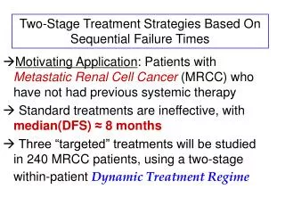
A Metastatic Renal Cancer Trial • Entry Criteria: Patients withMetastatic Renal Cell Cancer (MRCC) who have not had previous systemic therapy • Standard treatments are ineffective, with median(DFS) approximately 8 months Three “targeted” treatments will be studied in 240 MRCC patients, using a two-stage within-patient Dynamic Treatment Regime
A Within-Patient Two-Stage Treatment Assignment Algorithm (Dynamic Treatment Regime) Stage1 At entry, randomize the patient among the stage 1 treatment pool {A1,…,Ak} Stage 2 If the 1st failure is disease worsening (progression of MRCC) & not discontinuation, re-randomize the patient among a set of treatments {B1,…,Bn} not received initially “Switch-Away From a Loser”
Frontline Salvage Strategy A B C • B = (A, B) • C = (A, C) • A = (B, A) • C = (B, C) • A = (C, A) • B = (C, B)
Selection Trials: Screening New Treatments - Randomize patients among experimental treatment regimes E1,…, Ek - Evaluate each patient’s outcome(s) - Select the “best” treatment E[k] that maximizes a summary statistic quantifying treatment benefit A selection design does not test hypotheses It does not detect a given improvement over a null value with given test size and power E.g. with k=3, in the “null” case where q1 = q2 = q3 each Ej is selected with probability .33 (not .05 or some smaller value)
Goal of the Renal Cancer Trial Select the two-stage strategy having the largest “average” time to second treatment failure (“overall failure time”) With 6 strategies: In the “null” case where all strategies give the same overall failure time, each strategy is selected with probability 1/6 = .166
Higher Mathematics Stage1 treatment pool = {A1,…,Ak} Stage 2 treatment pool = {B1,…,Bn} kxn = # possible 2-stage strategies N/k = effective sample size to estimate each frontline rx effect N/(kn) = effective sample size to estimate each two-stage strategy effect
Higher Mathematics Example : If k=3, n=3 with “switch-away” within patient rule, and N=240 2x3 = 6 = # possible 2-stage strategies 240/3 = 80 = effective sample size to estimate each frontline rx effect 240/6 = 40 = effective sample size to estimate each two-stage strategy effect
Outcomes TD = time of discontinuation S1 = time from start of stage 1 of therapy of 1st disease worsening S2 = time from start of stage 2 of therapy to 2nd treatment failure d = delay between 1st progression and start of 2nd stage of treatment
Outcomes T1 = Time to 1st treatment failure T2 = Time from 1st disease worsening to 2nd treatment failure T1 + T2 = Time of 2nd treatment failure (provided that the 1st failure was not a discontinuation)
Unavoidable Complications Because disease is evaluated repeatedly (MRI, PET),either T1 or T1 + T2may be interval censored There may be a delay between 1st failure and start of stage 2 therapy T1 may affect T2 The failure rates may change over time (they increase for MRC)
Delay before start of 2nd stage rx Discontinuation Start of stage 2 rx
T2,1 = Time from 1st progression to 2nd treatment failure if it occurs during the delay interval before stage 2 therapy is begun T2,2 = Time from 1st progression to 2nd treatment failure if it occurs after stage 2 therapy has begun
A Simple Parametric Model Weib(a,x) = Weibull distribution with meanm(a,x) = ea G(1+e-x), for real-valued a and x [ T1 | A ] ~ Weib(aA,xA) [ T2,1 | A,B, T1] ~ Exp{ gA+bA log(T1) } [ T2,2 | A,B, T1] ~ Weib( gA,B+bA log(T1), xA,B)
Mean Overall Failure Time T = T1 + Y1,W T2 mA,B(q) = E{ T| (A,B)} = E(T1) + Pr(Y1,W =1) E(T2) Mean time to 1st failure Pr(1st failure is a Disease Worsening) Mean time to 2nd failure
Criteria for Choosing a Best Strategy Mean{ mA,B(q) | data }: B-Weib-Mean 2. Median{ mA,B(q) | data }: B-Weib-Median 3. MLE of mA,B(q) under simple Exponential: F-Exp-MLE 4. MLE of mA,B(q) under full Weibull: F-Weib-MLE
A Tale of Four Designs Design 1 (February 21, 2006) N=240, accrual rate a = 12/month 20 month accrual + 18 mos addt’l FU Stage 1 pool = {A,B,C,D} 12 strategies (A,B), (A,C), (A,D), (B,A), (B,C), (B,D), (C,A), (C,B), (C,D), (D,A), (D,B), (D,C) Drop-out rate .20 between stages (240/12) x .80 = 16 patients per strategy
A Tale of Four Designs Design 2 (April 17, 2006) Following “advice” from CTEP, NCI : N = 240, a = 9/month (“more realistic”) Stage 1 pool = {A,B} (C, D not allowed as frontline) Stage 2 pool = {A,B,C,D} 6 strategies : (A,B), (A,C), (A,D), (B,A), (B,C), (B,D) (240/6) x .80 = 32 patients per strategy
A Tale of Four Designs An Interesting Property of Design 2 Stage 1 may be thought of as a conventional phase III trial comparing A vs B with size .05 and power .80 to detect a 50% increase in median(T1), from 8 to 12 months, embedded in the two-stage design However, the design does not aim to test hypotheses. It is a selection design.
A Tale of Four Designs Design 3 (January 3, 2007) CTEP was no longer interested, but several Pharmas now VERY interested N = 360, a = 12/month, 3 new treatments Stage 1 rx pool = Stage 2 rx pool = {a,s,t} 6 strategies (different from Design 2) : (a,s), (a,t), (s,a), (s,t), (t,a), (t,s) (360/6) x .80 = 48 patients per strategy
A Tale of Four Designs Design 4 (May 15, 2007) Question: Should a futility stopping rule be included, in case the accrual rate turns out to be lower than planned? Answer: Yes!! “Weeding” Rule: When 120 pats. are fully evaluated, stop accrual to strategy (a,b) if Pr{ m(a,b) < m(best) – 3 mos | data} > .90
A Tale of Four Designs Applying the Weeding Rule when 120 patients have been fully evaluated
Establishing Priors q has 28 elements, but the 6 subvectors are qA,B= (n1,A, n2,A,B , aA , xA, gA, bA , aA,B , xA,B) Pr(Dis. Worsening)Reg. of T2 on T1 Weib pars of T1 Weib pars of T2 The qA,B’s are exchangeable across the 6 strategies, so they have the same priors
Establishing Priors n1,A ,n2,A,B~ iid beta(0.80, 0.20) based on clinical experience aA , xA, gA, bA , aA,B , xA,B ~ indep. normal priors Prior means: We elicited percentiles of T1 and [ T2 | T1 = 8 mos], & applied the Thall-Cook (2004) least squares method to determine means Prior variances: We set var{exp(aA)} = var{exp(xA)} = var{exp(xA,B)} = 100 Assuming Pr(Disc. During delay period) = .02 E(mA,B) = 7.0 mos & sd(mA,B) = 12.9
Computer Simulations Simulation Scenarios specified in terms of z1(A) = median (T1 | A) and z2(A,B) = median { T2,2 | T1 = 8, (A,B) } Null values z1 = 8 and z2 = 3 z1 = 12 Good frontline z2 = 6 Good salvage z2 = 9 Very good salvage
Simulations: No Weeding Rule In terms of the probabilities of correctly selecting superior strategies, F-Weib-MLE ~ B-Weib-Median > B-Weib-Mean >> F-Exp-MLE
Sims With Weeding Rule • Correct selection probabilities are affected only very slightly • There is a shift of patients from inferior strategies to superior strategies – but this only becomes substantial with lower accrual rates
Future Research / Extensions Distinguish betweendrop-out and other types of discontinuation and conduct “Informative Drop-Out” analysis Account forpatient heterogeneity Correct forselection biaswhen computing final estimates Accommodatemore than two stages