Download
1 / 66
670 likes | 938 Views
EEF011 Computer Architecture 計算機結構. Chapter 2 Instruction Set Principles and Examples. 吳俊興 高雄大學資訊工程學系 October 2004. Chapter 2. Instruction Set Principles and Examples. 2.1 Introduction 2.2 Classifying Instruction Set Architectures

E N D
EEF011 Computer Architecture計算機結構 Chapter 2Instruction Set Principles and Examples 吳俊興 高雄大學資訊工程學系 October 2004
Chapter 2. Instruction Set Principles and Examples 2.1 Introduction 2.2 Classifying Instruction Set Architectures 2.3 Memory Addressing 2.4 Addressing Modes for Signal Processing 2.5 Type and Size of Operands 2.6 Operands for Media and Signal Processing 2.7 Operations in the Instruction Set 2.8 Operations for Media and Signal Processing 2.9 Instructions for Control Flow 2.10 Encoding an Instruction Set
software instruction set hardware 2.1 Introduction Instruction Set Architecture – the portion of the machine visible to the assembly level programmer or to the compiler writer • In order to use the hardware of a computer, we must speak its language • The words of a computer language are called instructions, and its vocabulary is called an instruction set Instr. # Operation+Operands i movl -4(%ebp), %eax (i+1) addl %eax, (%edx) (i+2) cmpl 8(%ebp), %eax (i+3) jl L5 : L5:
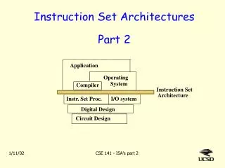
Topics • A taxonomy of instruction set alternatives and qualitative assessment • Instruction set quantitative measurements • Specific instruction set architecture • Issues and bearings of languages and compilers • Examples: MIPS and Trimedia TM32 CPU Appendices C-F: MIPS, PowerPC, Precision Architecture, SPARC ARM, Hitachi SH, MIPS 16, Thumb 80x86 (App. D),IBM 360/370 (App. E), VAX (App. F)
2.2 Classifying Instruction Set Architectures These choices critically affect number of instructions, CPI, and CPU cycle time
ISA Classification • Most basic differentiation: internal storage in a processor • Operands may be named explicitly or implicitly • Major choices: • In an accumulator architecture one operand is implicitly the accumulator => similar to calculator • The operands in a stack architecture are implicitly on the top of the stack • The general-purpose register architectures have only explicit operands – either registers or memory location
Basic ISA Classes Register-register, register-memory, and memory-memory (gone) options
Example Stack: 0 address add tos ¬ tos + next Accumulator: 1 address add A acc ¬ acc + mem[A] General Purpose Register (register-memory): 1 address add R1 A R1 ¬ R1 + mem[A] GPR (register-register or called load/store): 0 address load R1, A R1 ¬ mem[A] load R2, B R2 ¬ mem[B] add R3, R1, R2 R3 ¬ R1+R2 ALU Instructions can have two operands. ALU Instructions can have three operands.
Pro’s and Con’s Register is the class that won out!
Register Machines • How many registers are sufficient? • General-purpose registers vs. special-purpose registers • compiler flexibility and hand-optimization • Two major concerns for arithmetic and logical instructions (ALU) • 1. Two or three operands • X + Y X • X + Y Z • 2. How many of the operands may be memory addresses (0 – 3) Hence, register classification (# mem, # operands)
(0, 3): Register-Register • ALU is Register to Register – also known as • pureReduced Instruction Set Computer (RISC) • Advantages • simple fixed length instruction encoding • decode is simple since instruction types are small • simple code generation model • instruction CPI tends to be very uniform • • except for memory instructions of course • • but there are only 2 of them - load and store • Disadvantages • instruction count tends to be higher • some instructions are short - wasting instruction word bits
(1, 2): Register-Memory • Evolved RISC and also old CISC • • new RISC machines capable of doing speculative loads • • predicated and/or deferred loads are also possible • Advantages • data access to ALU immediate without loading first • instruction format is relatively simple to encode • code density is improved over Register (0, 3) model • Disadvantages • operands are not equivalent - source operand may be destroyed • need for memory address field may limit # of registers • CPI will vary • • if memory target is in L0 cache then not so bad • • if not - life gets miserable
(2, 2) or (3, 3): Memory-Memory • True and most complex CISC model • • currently extinct and likely to remain so • • more complex memory actions are likely to appear but not • directly linked to the ALU • Advantages • most compact code • doesn’t waste registers for temporary values • good idea for use once data - e.g. streaming media • Disadvantages • large variation in instruction size - may need a shoe-horn • large variation in CPI - i.e. work per instruction • exacerbates the infamous memory bottleneck • register file reduces memory accesses if reused • Not used today
2.3 Memory Addressing • In today’s machine, objects have byte addresses – an address refers to the number of bytes counted from the beginning of memory • Object Length: Provides access for bytes (8 bits), half words (16 bits), words (32 bits), and double words (64 bits). The type is implied in opcode (e.g., LDB – load byte; LDW – load word; etc.) • Byte Ordering • Little Endian: puts the byte whose address is xx00 at the least significant position in the word. (7,6,5,4,3,2,1,0) • Big Endian: puts the byte whose address is xx00 at the most significant position in the word. (0,1,2,3,4,5,6,7) • Problem occurs when exchanging data among machines with different orderings Interpreting Memory Addresses
Interpreting Memory Addresses • Alignment Issues • Accesses to objects larger than a byte must be aligned. An access to an object of size s bytes at byte address A is aligned if A mod s = 0. • Misalignment causes hardware complications, since the memory is typically aligned on a word or a double-word boundary • Misalignment typically results in an alignment fault that must be handled by the OS • Hence • • byte address is anything - never misaligned • • half word - even addresses - low order address bit = 0 ( XXXXXXX0) else trap • • word - low order 2 address bits = 0 ( XXXXXX00) else trap • • double word - low order 3 address bits = 0 (XXXXX000) else trap
Addressing Modes How do architectures specify the addr. of an object they will access? • Effective address: the actual memory address specified by the addressing mode. • “->” is for assignment. Mem[R[R1]] refers to the contents of the memory location whose location is given the contents of register 1 (R1).
Figure 2.7 Summary of use of memory addressing modes Based on a VAX which supported everything – from SPEC89
Displacement Addressing Mode How big should the displacement be? Figure 2.8 Displacement values are widely distributed
Displacement Addressing Mode (cont.) • Benchmarks show 12 bits of displacement would capture about 75% of the full 32-bit displacements and 16 bits should capture about 99% • Remember: optimize for the common case. Hence, the choice is at least 12-16 bits • For addresses that do fit in displacement size: • Add R4, 10000 (R0) • For addresses that don’t fit in displacement size, the compiler must do the following: Load R1, 1000000 Add R1, R0 Add R4, 0 (R1)
Immediate Addressing Mode • Used where we want to get to a numerical value in an instruction • Around 20% of the operations have an immediate operand At high level: a = b + 3; if ( a > 17 ) goto Addr At Assembler level: Load R2, 3 Add R0, R1, R2 Load R2, 17 CMPBGT R1, R2 Load R1, Address Jump (R1)
Immediate Addressing Mode How frequent for immediates? Figure 2.9 About one-quarter of data transfers and ALU operations have an immediate operand
Immediate Addressing Mode How big for immediates? Figure 2.10 Benchmarks show that 50%-70% of the immediates fit within 8 bits and 75%-80% fit within 16 bits
2.4 Addressing Modes for Signal Processing Two addressing modes that distinguish DSPs • Modulo or circular addressing mode • autoincrement/autodecrement to support circular buffers • As data are added, a pointer is checked to see if it is pointing to the end of the buffer • If not, the pointer is incremented to the next address • If it is, the pointer is set instead to the start of the buffer • Bit reverse addressing mode • the hardware reverses the lower bits of the address, with the number of bits reversed depending on the step of the FFT algorithm
Addressing for Fast Fourier Transform (FFT) • FFTs start or end their processing with data shuffled in a particular order Without special support, such address transformations would take an extra memory access to get the new address, or involve a fair amount of logical instructions to transform the address
Figure 2.11 Static Frequency of Addressing Modes for TI TMS320C54x DSP 17 addressing modes, 6 modes also found in Figure 2.6 account for 95% of the DSP addressing
Summary: Memory Addressing • A new architecture expected to support at least: displacement, immediate, and register indirect • represent 75% to 99% of the addressing modes (Figure 2.7) • The size of the address for displacement mode to be at least 12-16 bits • capture 75% to 99% of the displacements (Figure 2.8) • The size of the immediate field to be at least 8-16 bits • capture 50% to 80% of the immediates (Figure 2.10) Desktop and server processors rely on compilers, but historically DSPs rely on hand-coded libraries
2.5 Type And Size of Operands How is the type of an operand designated? • The type of the operand is usually encoded in the opcode • e.g., LDB – load byte; LDW – load word • Common operand types: (imply their sizes) Character (8 bits or 1 byte) Half word (16 bits or 2 bytes) Word (32 bits or 4 bytes) Double word (64 bits or 8 bytes) Single precision floating point (4 bytes or 1 word) Double precision floating point (8 bytes or 2 words) • Characters are almost always in ASCII • 16-bit Unicode (used in Java) is gaining popularity • Integers are two’s complement binary • Floating points follow the IEEE standard 754 • Some architectures support packed decimal: 4 bits are used to encode the values 0-9; 2 decimal digits are packed into each byte
Figure 2.12 Distribution of data accesses by size for the benchmark programs SPEC2000 Operand Sizes The double-word data type is used for double-precision floating point in floating-point programs and for addresses
2.6 Operands for Media and Signal Processing • Vertex • A common 3D data type dealt in graphics applications • four components: (x, y, z) and w=color or hidden surfaces • vertex values are usually 32-bit floating-point values • Three vertices specify a graphics primitive such as a triangle • Pixel • Typically 32 bits, consisting of four 8-bit channels • R (red), G (green), B (blue), and A (attribute: eg. transparency) • DSPs add fixed point • fractions between -1 and +1 (divide by 2n-1) • Blocked floating point • a block of variables with common exponent • accumulators, registers that are wider to guard against round-off error to aid accuracy in fixed-point arithmetic
Size of Data operands for DSP Figure 2.13 Four generations of DSPs, their data width, and the width of the registers that reduces round-off error Figure 2.14 Size of data operands for TMS320C540x DSP. This DSP has two 40-bit accumulators and no floating-point operations.
Brief Summary • Review instruction set classes • choose register-register class • Review memory addressing • select displacement, immediate, and register indirect addressing modes • Select the operand sizes and types
2.7 Operations in the Instruction Set Figure 2.15 Categories of instruction operators and examples of each. • All computers generally provide a full set of operations for the first three categories • All computers must have some instruction support for basic system functions • Graphics instructions typically operate on many smaller data items in parallel
Figure 2.16 Top 10 instructions for the 80x86 • Simple instructions dominate this list and responsible for 96% of the instructions executed • These percentages are the average of the five SPECint 92 programs
2.8 Operations for Media & Signal Processing • Data for multimedia operations is often narrower than the 64-bit data word • normally in single precision, not double precision • Single-instruction multiple-data (SIMD) or vector instructions • A partitioned add operation on 16-bit data with a 64-bit ALU would perform four 16-bit adds in a single clock cycle • Hardware cost: prevent carries between the four 16-bit partitions of the ALU • Two 32-bit floating-point operations (paired single operations) • The two partitions must be insulated to prevent operations on one half from affecting the other
Figure 2.17 Summary of multimedia support for desktop RISCs • B: byte (8 bits), H: half word (16 bits), W: word (32 bits) 8B: operation on 8 bytes in a single instruction • All are fixed-width operations, performing multiple narrow operations on either a 64-bit or 128-bit ALU
Multimedia Operations for DSPs • DSP architectures use saturating arithmetic • If the result is too large to be represented, it is set to the largest representable number • There is not an option of causing an exception on arithmetic overflow • Prevent missing an event in real-time applications • The result will be used no matter what the inputs • There are several modes to round the wider accumulators into the narrower data words • The targeted kernels for DSPs accumulate a series of produces, and hence have a multiply-accumulate (MAC) instruction • MACs are key to dot product operations for vector and matrix multiplies • Finite Impulse Response (FIR) Problem • y[n] = S c[k] * x[n-k] • In C: • y[n] = 0 • for(k=0; k <N; k++) • y[n] = y[n] + c[k]*x[n-k] • General form: • x = x + y * z • IBM PowerPC 440 MAC instruction: • macchw RT, RA, RB • where RT = x, RA = y, RB = z
Figure 2.18 Mix of instructions for TMS320C540x DSP • 16-bit architecture use two 40-bit accumulators, 8 address registers, no floating-point operations (fixed points instead), plus a stack for passing parameters to library routines and for saving return addresses • 15% to 20% of the multiplies and MACs round the final sum (not shown)
2.9 Instructions for Control Flow • Control instructions change the flow of control: instead of executing the next instruction, the program branches to the address specified in the branching instructions • They are a big deal • Primarily because they are difficult to optimize out • AND they are frequent • Four types of control instructions • Conditional branches • Jumps – unconditional transfer • Procedure calls • Procedure returns
Control Flow Instructions • Issues: • Where is the target address? How to specify it? • Where is return address kept? How are the arguments passed? (calls) • Where is return address? How are the results passed? (returns) • Figure 2.19 Breakdown
Addressing Modes for Control Flow Instructions • PC-relative (Program Counter) • supply a displacement added to the PC • Known at compile time for jumps, branches, and calls (specified within the instruction) • the target is often near the current instruction • requiring fewer bits • independently of where it is loaded (position independence) • Register indirect addressing – dynamic addressing • The target address may not be known at compile time • Naming a register that contains the target address • Case or switch statements • Virtual functions or methods • High-order functions or function pointers • Dynamically shared libraries
Figure 2.20 Branch distances These measurements were taken on a load-store computer (Alpha architecture) with all instructions aligned on word boundaries
Conditional Branch Options Figure 2.21 Major methods for evaluating branch conditions
Figure 2.22 Comparison Type vs. Frequency • Most loops go from 0 to n. • Most backward branches are loops – taken about 90%
Repeat Instruction for DSP • DSPs: add looping structure, called a repeat instruction, to avoid loop overhead • It allows a single instruction or a block of instructions to be repeated up to, say, 256 times • eg. TMS320C54 dedicates three special registers to hold the block starting address, ending address, and repeat counter
Procedure Invocation Options • Procedure calls and returns • control transfer • state saving; the return address must be saved Newer architectures require the compiler to generate stores and loads for each register saved and restored • Two basic conventions in use to save registers • caller saving: the calling procedure must save the registers that it wants preserved for access after the call • the called procedure need not worry about registers • callee saving: the called procedure must save the registers it wants to use • leaving the caller unrestrained most real systems today use a combination of the two mechanisms • specified in an application binary interface (ABI) that set down the basic rules as to which register be caller saved and which should be callee saved
2.10 Encoding an Instruction Set • Opcode: specifying the operation • # of operand • addressing mode • address specifier: tells what addressing mode is used • Load-store computer • Only one memory operand • Only one or two addressing modes • Encoding issues • The desire to have as many registers and addressing modes as possible • The impact of the size of the register and addressing mode fields on the average instruction size and hence on the average program size • A desire to have instructions encoded into lengths that will be easy to handle in a pipelined implementation Figure 2.23 Three basic variations in instruction encoding • The length of 80x86 instructions varies between 1 and 17 bytes • Trade-off: size of programs vs. ease of decoding
Reduced Code Size in RISCs • Hybrid encoding – support 16-bit and 32-bit instructions in RISC, eg. ARM Thumb and MIPS 16 • narrow instructions support fewer operations, smaller address and immediate fields, fewer registers, and two-address format rather than the classic three-address format • claim a code size reduction of up to 40% • Compression in IBM’s CodePack • Adds hardware to decompress instructions as they are fetched from memory on an instruction cache miss • The instruction cache contains full 32-bit instructions, but compressed code is kept in main memory, ROMs, and the disk • Hitachi’s SuperH: fixed 16-bit format • 16 rather than 32 registers • fewer instructions