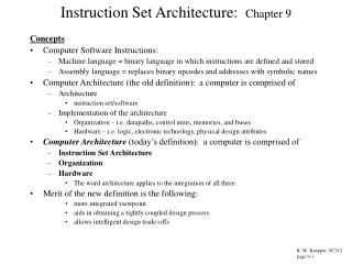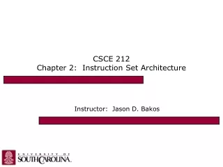
Chapter 2 Instruction Set Principles
Chapter 2 Instruction Set Principles. Computer Architecture’s Changing Definition. 1950s to 1960s: Computer Architecture Course = Computer Arithmetic 1970s to mid 1980s: Computer Architecture Course = Instruction Set Design, especially ISA appropriate for compilers

Chapter 2 Instruction Set Principles
E N D
Presentation Transcript
Computer Architecture’s Changing Definition • 1950s to 1960s: Computer Architecture Course = Computer Arithmetic • 1970s to mid 1980s: Computer Architecture Course = Instruction Set Design, especially ISA appropriate for compilers • 1990s: Computer Architecture Course = Design of CPU, memory system, I/O system, Multiprocessors
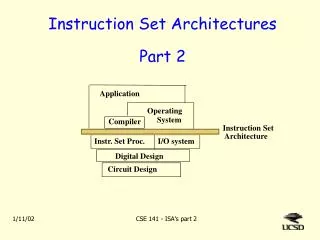
Instruction Set Architecture (ISA) software instruction set hardware
Instruction Set Architecture • Instruction set architecture is the structure of a computer that a machine language programmer must understand to write a correct (timing independent) program for that machine. • The instruction set architecture is also the machine description that a hardware designer must understand to design a correct implementation of the computer.
Interface Design • A good interface: • Lasts through many implementations (portability, compatibility) • Is used in many different ways (generality) • Provides convenient functionality to higher levels • Permits an efficient implementation at lower levels use time imp 1 Interface use imp 2 use imp 3
Evolution of Instruction Sets Single Accumulator (EDSAC 1950) Accumulator + Index Registers (Manchester Mark I, IBM 700 series 1953) Separation of Programming Model from Implementation High-level Language Based Concept of a Family (B5000 1963) (IBM 360 1964) General Purpose Register Machines Complex Instruction Sets Load/Store Architecture (CDC 6600, Cray 1 1963-76) (Vax, Intel 432 1977-80) RISC (Mips,Sparc,HP-PA,IBM RS6000,PowerPC . . .1987) LIW/”EPIC”? (IA-64. . .1999)
Evolution of Instruction Sets • Major advances in computer architecture are typically associated with landmark instruction set designs • Ex: Stack vs GPR (System 360) • Design decisions must take into account: • technology • machine organization • programming languages • compiler technology • operating systems • And they in turn influence these
What Are the Components of an ISA? • Sometimes known as The Programmer’s Model of the machine • Storage cells • General and special purpose registers in the CPU • Many general purpose cells of same size in memory • Storage associated with I/O devices • The machine instruction set • The instruction set is the entire repertoire of machine operations • Makes use of storage cells, formats, and results of the fetch/execute cycle • i.e., register transfers
What Are the Components of an ISA? • The instruction format • Size and meaning of fields within the instruction • The nature of the fetch-execute cycle • Things that are done before the operation code is known
What Must an Instruction Specify?(I) Data Flow • Which operation to perform add r0, r1, r3 • Ans: Op code: add, load, branch, etc. • Where to find the operands: add r0, r1, r3 • In CPU registers, memory cells, I/O locations, or part of instruction • Place to store result add r0, r1, r3 • Again CPU register or memory cell
What Must an Instruction Specify?(II) • Location of next instruction add r0, r1, r3 br endloop • Almost always memory cell pointed to by program counter—PC • Sometimes there is no operand, or no result, or no next instruction. Can you think of examples?
Instructions Can Be Divided into 3 Classes (I) • Data movement instructions • Move data from a memory location or register to another memory location or register without changing its form • Load—source is memory and destination is register • Store—source is register and destination is memory • Arithmetic and logic (ALU) instructions • Change the form of one or more operands to produce a result stored in another location • Add, Sub, Shift, etc. • Branch instructions (control flow instructions) • Alter the normal flow of control from executing the next instruction in sequence • Br Loc, Brz Loc2,—unconditional or conditional branches
Classifying ISAs Accumulator (before 1960): 1 address add A acc <-acc + mem[A] Stack (1960s to 1970s): 0 address add tos <-tos + next Memory-Memory (1970s to 1980s): 2 address add A, B mem[A] <-mem[A] + mem[B] 3 address add A, B, C mem[A] <-mem[B] + mem[C] Register-Memory (1970s to present): 2 address add R1, A R1 <-R1 + mem[A] load R1, A R1 <_mem[A] Register-Register (Load/Store) (1960s to present): 3 address add R1, R2, R3 R1 <-R2 + R3 load R1, R2 R1 <- mem[R2] store R1, R2 mem[R1] <-R2
Stack Architectures • Instruction set: add, sub, mult, div, . . . push A, pop A • Example: A*B - (A+C*B) push A push B mul push A push C push B mul add sub A C B B*C A+B*C result A B A*B A*B A C A A*B A A*B A A*B A*B
Stacks: Pros and Cons • Pros • Good code density (implicit operand addressing top of stack) • Low hardware requirements • Easy to write a simpler compiler for stack architectures • Cons • Stack becomes the bottleneck • Little ability for parallelism or pipelining • Data is not always at the top of stack when need, so additional instructions like TOP and SWAP are needed • Difficult to write an optimizing compiler for stack architectures
Accumulator Architectures • Instruction set: • add A, sub A, mult A, div A, . . . • load A, store A • Example: A*B - (A+C*B) • load B • mul C • add A • store D • load A • mul B • sub D B B*C A+B*C A+B*C A A*B result
Accumulators: Pros and Cons • Pros • Very low hardware requirements • Easy to design and understand • Cons • Accumulator becomes the bottleneck • Little ability for parallelism or pipelining • High memory traffic
Memory-Memory Architectures • Instruction set: • (3 operands) add A, B, C sub A, B, C mul A, B, C • Example: A*B - (A+C*B) • 3 operands • mul D, A, B • mul E, C, B • add E, A, E • sub E, D, E
Memory-Memory:Pros and Cons • Pros • Requires fewer instructions (especially if 3 operands) • Easy to write compilers for (especially if 3 operands) • Cons • Very high memory traffic (especially if 3 operands) • Variable number of clocks per instruction (especially if 2 operands) • With two operands, more data movements are required
Register-Memory Architectures • Instruction set: • add R1, A sub R1, A mul R1, B • load R1, A store R1, A • Example: A*B - (A+C*B) • load R1, A • mul R1, B /* A*B */ • store R1, D • load R2, C • mul R2, B /* C*B */ • add R2, A /* A + CB */ • sub R2, D /* AB - (A + C*B) */
Memory-Register: Pros and Cons • Pros • Some data can be accessed without loading first • Instruction format easy to encode • Good code density • Cons • Operands are not equivalent (poor orthogonality) • Variable number of clocks per instruction • May limit number of registers
Load-Store Architectures • Instruction set: • add R1, R2, R3 sub R1, R2, R3 mul R1, R2, R3 • load R1, R4 store R1, R4 • Example: A*B - (A+C*B) • load R1, &A • load R2, &B • load R3, &C • load R4, R1 • load R5, R2 • load R6, R3 • mul R7, R6, R5 /* C*B */ • add R8, R7, R4 /* A + C*B */ • mul R9, R4, R5 /* A*B */ • sub R10, R9, R8 /* A*B - (A+C*B) */
Load-Store: Pros and Cons • Pros • Simple, fixed length instruction encoding • Instructions take similar number of cycles • Relatively easy to pipeline • Cons • Higher instruction count • Not all instructions need three operands • Dependent on good compiler
Registers:Advantages and Disadvantages • Advantages • Faster than cache (no addressing mode or tags) • Deterministic (no misses) • Can replicate (multiple read ports) • Short identifier (typically 3 to 8 bits) • Reduce memory traffic • Disadvantages • Need to save and restore on procedure calls and context switch • Can’t take the address of a register (for pointers) • Fixed size (can’t store strings or structures efficiently) • Compiler must manage
C P U I n s t r u c t i o n f o r m a t s R e g i s t e r s M e m o r y l o a d R 8 , O p 1 ( R 8 ฌ O p 1 ) l o a d R 8 O p 1 A d d r : O p 1 l o a d R 8 O p 1 A d d r R 6 R 4 a d d R 2 , R 4 , R 6 ( R 2 ฌ R 4 + R 6 ) a d d R 2 R 4 R 6 R 2 P r o g r a m N e x t i c o u n t e r General Register Machine and Instruction Formats
General Register Machine and Instruction Formats • It is the most common choice in today’s general-purpose computers • Which register is specified by small “address” (3 to 6 bits for 8 to 64 registers) • Load and store have one long & one short address: One and half addresses • Arithmetic instruction has 3 “half” addresses
Real Machines Are Not So Simple • Most real machines have a mixture of 3, 2, 1, 0, and 1- address instructions • A distinction can be made on whether arithmetic instructions use data from memory • If ALU instructions only use registers for operands and result, machine type is load-store • Only load and store instructions reference memory • Other machines have a mix of register-memory and memory-memory instructions
Alignment Issues • If the architecture does not restrict memory accesses to be aligned then • Software is simple • Hardware must detect misalignment and make 2 memory accesses • Expensive detection logic is required • All references can be made slower • Sometimes unrestricted alignment is required for backwards compatibility • If the architecture restricts memory accesses to be aligned then • Software must guarantee alignment • Hardware detects misalignment access and traps • No extra time is spent when data is aligned • Since we want to make the common case fast, having restricted alignment is often a better choice, unless compatibility is an issue
Types of Addressing Modes (VAX) memory 1. Register direct Ri 2. Immediate (literal) #n 3. Displacement M[Ri + #n] 4. Register indirect M[Ri] 5. Indexed M[Ri + Rj] 6. Direct (absolute) M[#n] 7. Memory Indirect M[M[Ri] ] 8. Autoincrement M[Ri++] 9. Autodecrement M[Ri - -] 10. Scaled M[Ri + Rj*d + #n] reg. file
Types of Operations • Arithmetic and Logic: AND, ADD • Data Transfer: MOVE, LOAD, STORE • Control BRANCH, JUMP, CALL • System OS CALL, VM • Floating Point ADDF, MULF, DIVF • Decimal ADDD, CONVERT • String MOVE, COMPARE • Graphics (DE)COMPRESS
Control instructions (contd.) • Addressing modes • PC-relative addressing (independent of program load & displacements are close by) • Requires displacement (how many bits?) • Determined via empirical study. [8-16 works!] • For procedure returns/indirect jumps/kernel traps, target may not be known at compile time. • Jump based on contents of register • Useful for switch/(virtual) functions/function ptrs/dynamically linked libraries etc.
Frequency of Different Types of Compares in Conditional Branches
Encoding an Instruction set • a desire to have as many registers and addressing mode as possible • the impact of size of register and addressing mode fields on the average instruction size and hence on the average program size • a desire to have instruction encode into lengths that will be easy to handle in the implementation
Compilers and ISA • Compiler Goals • All correct programs compile correctly • Most compiled programs execute quickly • Most programs compile quickly • Achieve small code size • Provide debugging support • Multiple Source Compilers • Same compiler can compiler different languages • Multiple Target Compilers • Same compiler can generate code for different machines
Compiler Based Register Optimization • Assume small number of registers (16-32) • Optimizing use is up to compiler • HLL programs have no explicit references to registers • usually – is this always true? • Assign symbolic or virtual register to each candidate variable • Map (unlimited) symbolic registers to real registers • Symbolic registers that do not overlap can share real registers • If you run out of real registers some variables use memory
Graph Coloring • Given a graph of nodes and edges • Assign a color to each node • Adjacent nodes have different colors • Use minimum number of colors • Nodes are symbolic registers • Two registers that are live in the same program fragment are joined by an edge • Try to color the graph with n colors, where n is the number of real registers • Nodes that can not be colored are placed in memory
Allocation of Variables • Stack • used to allocate local variables • grown and shrunk on procedure calls and returns • register allocation works best for stack-allocated objects • Global data area • used to allocate global variables and constants • many of these objects are arrays or large data structures • impossible to allocate to registers if they are aliased • Heap • used to allocate dynamic objects • heap objects are accessed with pointers • never allocated to registers
Designing ISA to Improve Compilation • Provide enough general purpose registers to ease register allocation ( more than 16). • Provide regular instruction sets by keeping the operations, data types, and addressing modes orthogonal. • Provide primitive constructs rather than trying to map to a high-level language. • Simplify trade-off among alternatives. • Allow compilers to help make the common case fast.
ISA Metrics • Orthogonality • No special registers, few special cases, all operand modes available with any data type or instruction type • Completeness • Support for a wide range of operations and target applications • Regularity • No overloading for the meanings of instruction fields • Streamlined Design • Resource needs easily determined. Simplify tradeoffs. • Ease of compilation (programming?), Ease of implementation, Scalability