Download
1 / 38
380 likes | 581 Views
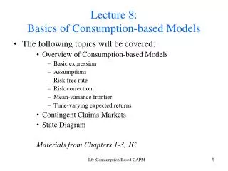
Lecture 8: Basics of Consumption-based Models. The following topics will be covered: Overview of Consumption-based Models Basic expression Assumptions Risk free rate Risk correction Mean-variance frontier Time-varying expected returns Contingent Claims Markets State Diagram

E N D
Lecture 8: Basics of Consumption-based Models • The following topics will be covered: • Overview of Consumption-based Models • Basic expression • Assumptions • Risk free rate • Risk correction • Mean-variance frontier • Time-varying expected returns • Contingent Claims Markets • State Diagram Materials from Chapters 1-3, JC L8: Consumption Based CAPM
General Info • Lucas (1978) introduced the consumption-based asset pricing model • In it, an economic agent chooses consumption and investment strategies over discrete time periods during an infinite life so as to maximize expected utility. • Hansen (1982) and Hansen and Singleton (1982) introduced GMM to test the model L8: Consumption Based CAPM
Stochastic Discount Factor Presentation L8: Consumption Based CAPM
Stochastic Discount Factor L8: Consumption Based CAPM
Bellman Approach – A More General Approach • W is wealth • E is endowment • c is consumption • d is for discount • Objective Function L8: Consumption Based CAPM
Bellman Approach • Additive utility U(c) • Principle of optimality: An optimal policy has the property that whatever the initial state and initial decision are, the remaining decisions must constitute an optimal policy with regard to the state resulting from the first decision. • The maximum remaining utility at time t is then written as L8: Consumption Based CAPM
Bellman Equation L8: Consumption Based CAPM
Relation with AD Assets • How to express the price of a security? • What is the risk free rate? • What determines state price per unit of probability? L8: Consumption Based CAPM
Examples: p=E(mx) Asset price Stock return Excess stock return Risk free rate See page 9 – 10 of Cochrane. Note: L8: Consumption Based CAPM
Assumptions Not Used • Markets are complete, or there is a representative investor • Asset returns or payoffs are normally distributed, or independent over time • 2-period investors, quadratic utility, or separable utility • Investors have no human capital or labor income • The market has reached equilibrium, or investors have bought all the securities they want to • The assumption being made is: investor can consider a small marginal investment or disinvestment. L8: Consumption Based CAPM
Risk-free rate L8: Consumption Based CAPM
Risk Corrections The first term is the present value of E(x) (expected payoff). The second is a risk adjustment. An asset whose payoff co-varies positively with the discount factor has its price raised and vice versa. The key u’(c) is inversely related to c. If you buy an asset whose payoff covaries negatively with consumption (hence u’(c)), it helps to smooth consumption and so is more valuable than its expected payoff indicates. L8: Consumption Based CAPM
Risk Corrections – Return Expression All assets have an expected return equal to the risk-free rate, plus a risk adjustment. Assets whose returns covary positively with consumption make consumption more volatile, and so must promise higher expected returns to induce investor to hold them, and vice versa. L8: Consumption Based CAPM
Idiosyncratic Risk Does Not Affect Prices • That is, as long as cov(m,x)=0, then • Only systematic risk generates a risk correction. • Decomposition: x = proj(x|m) + ε: the first part of the projection on m. L8: Consumption Based CAPM
Expected Return-Beta Representation Where βis the regression coefficient of the asset return on m. It says each expcted return should be proportional to the regression coefficient in a regression of that return on the discount factor m. λis interpreted as the price of risk and β is the quantity of risk in each asset. L8: Consumption Based CAPM
Mean-Variance Frontier • Implications: • Means and variances of asset returns lie within efficient frontier. • On the efficient frontier, returns are perfectly correlated with the discount factor – interesting point! • The priced return is perfectly correlated with the discount factor and hence perfectly correlated with any frontier return. The residual generates no expected return. L8: Consumption Based CAPM
Mean Variance Frontier (Cont’d) • All frontier are perfectly correlated with each other since they are all perfectly correlated with the discount factor. This fact implies that we can span or synthesize any frontier return from two such returns. • We can have a single beta representation: • We can decompose returns into a “priced” or “systematic” component and a “residual” component as shown in the figure. The priced part is perfectly correlated with the discount factor. The residual part generates no expected return. L8: Consumption Based CAPM
Sharpe Ratio Let Rmv denote the return of a portfolio on the mean-variance efficient frontier and consider power utility. The slope of the frontier (Sharpe ratio) is Sharpe ratio is higher if consumption is more volatile or if investors are more risk averse. L8: Consumption Based CAPM
Equity Premium Puzzle • Over the last 50 years, average real stock return is 9% with a standard deviation of 16%. The real risk free rate is 1%. This suggests a real Sharpe ratio of _____ • Aggregate nondurable and services consumption growth has a standard deviation of 1%. So L8: Consumption Based CAPM
Time-varying Expected Returns The relation above is conditional. Conditional mean or other moment of a random variable could be different from its unconditional moment. E.g,, knowing tonight’s weather forecast, you can better predict rain tomorrow than just knowing the average rain for that date. It suggests a link between conditional mean of stock returns and conditional variance of stock returns. Little empirical support. L8: Consumption Based CAPM
Present-Value Statement • We can write out the long term objective as: • An investor can purchase a stream {dt+j} at price pt. • Then we have the first order condition as: L8: Consumption Based CAPM
Present-Value Statement • We can write a risk adjustment to price as the below: • Cover CLM Chapter 7.1 – Present Value Relation (page 253-267) L8: Consumption Based CAPM
Discount Factors in Continuous Time • Let a generic security have price pt at any moment in time, and let it pay dividends at the rate Dt. • The instantaneous total return is: • The utility function is: • Suppose the investor can buy a security whose price is pt and that pays a dividend stream Dt. L8: Consumption Based CAPM
Discount Factors in Continuous Time • The first-order condition for this problem gives us the infinite-period version of the basic pricing equation: • Define the “discount factor” in continuous time as • The pricing equation is: L8: Consumption Based CAPM
Continuous Time Model • The analogue to the one-period pricing equation p=E(mx) is: • This is no longer price equal to future value expression • Basically this is equivalent to: L8: Consumption Based CAPM
Continuous Time Model • With Ito Lemma, • This is the continuous-time analogue to L8: Consumption Based CAPM
Continuous Time Model • With: • Applying Ito Lemma (page 495), we have: L8: Consumption Based CAPM
General Equilibrium • Alternative ways in specifying the equilibrium • Solution 1 (linear technology model): the real, physical rate of return (the rate of intertemporal transformation) is not affected by how much is invested. Consumption must adjust to the technologically given rates of return. • CAPM; ICAPM; Cox, Ingersoll and Ross (1985) • Solution 2 (endowment economy): nondurable consumption appears every period. Hence, asset prices must adjust until people are just happy consuming the endowment process. • Lucas (1978); Mehra and Prescott (1985) • Solution 3 (concave technology): see Figure 2.3, page 40, JC L8: Consumption Based CAPM
Consumption-Based Model in Practice • Consider a standard power utility function: • Excess return should obey: • Apply covariance decomposition, we have: • We can verify the holding of the above equality. • Not much support. Page 43, JC. L8: Consumption Based CAPM
Alternative Asset Pricing Models • Different utility functions • General equilibrium models • Factor pricing models • Arbitrage or near-arbitrage pricing L8: Consumption Based CAPM
Contingent Claim: A review • page 50, JC Here, m is regarding states. L8: Consumption Based CAPM
Risk-Neutral Probabilities • Define: • E* is the expectation under risk neutral probability L8: Consumption Based CAPM
Utility Maximization • Budget constraint: total consumption equates total income • see page 53, JC. Marginal rate of substitution between states tomorrow equals the relevant price ratio. L8: Consumption Based CAPM
State Diagram and Price Function • The above represents a 2-state diagram. I.e., s=1,2. • Two axes represent payoffs in two states. pc vector is for unit state price. • All points in price =p (return) line or plane represent state payoff combinations yielding the same security price. • Risk free rate is on price=1 line. Why? L8: Consumption Based CAPM
State Diagram and Price Function • Think of contingent claims price pc and asset payoffs as vectors in Rs, where each element gives the price or payoff to the corresponding state. • We have the state diagram • The contingent claims price vector pc points into the positive orthant. • The set of payoffs with any given price lie on a (hyper)plane perpendicular to the contingent claim price vector. • Planes of constant price move out linearly, and the orgin x=0 must have a price of zero. • Inner product L8: Consumption Based CAPM
Exercises • 1.1; 1.5; 1.7 (JC) • Prove the expression for proj(x|m) • 2.2 (JC) L8: Consumption Based CAPM