Face recognition and detection using Principal Component Analysis PCA
680 likes | 1.02k Views
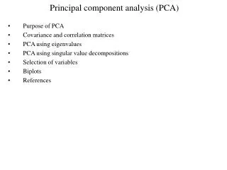
Face recognition and detection using Principal Component Analysis PCA. KH Wong. Overview. PCA P rinciple C omponent A nalysis Application to face detection and recognition Reference: [Bebis ] Applications 1) Face detection 2) Face recognition. PCA Principle component analysis [1].

Face recognition and detection using Principal Component Analysis PCA
E N D
Presentation Transcript
Face recognition and detection using Principal Component Analysis PCA KH Wong Face recognition & detection using PCA v.3f
Overview • PCA Principle Component Analysis • Application to face detection and recognition • Reference: [Bebis ] • Applications • 1) Face detection • 2) Face recognition Face recognition & detection using PCA v.3f
PCA Principle component analysis [1] • A method of data compression • Use less data in “b” to represent ‘”a” but retain important information • E.g N=10, 10 dimensions reduced to K=5 dimensions. • The task is to identify the N important parameters. • So recognition is easier. A detailed Christmas tree: N parameters A rough Christmas tree with K important parameters, where N>K. Face recognition & detection using PCA v.3f
Data reduction N dataK data (N>K), how? k N N k Face recognition & detection using PCA v.3f
Dimensionality basis Face recognition & detection using PCA v.3f
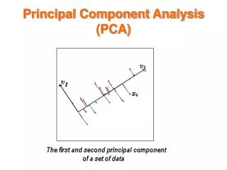
Condition for data reduction:data must not be random Data reduction (Compression) is difficult for random data Compression is easy for non-random data u1 x2 x2 x1 x1 Data are spread all over the 2D space, so redundancy of using 2 axes (x1,x2) is low Data are spread along one line , so redundancy of using 2 axes is high. Can consider to use one axis (U1) along the spread of data to represent it. Although some error may be introduced. Face recognition & detection using PCA v.3f
u2 v1 u1 The concept u2 • In this diagram, the data is not entirely random. • Transform the data from (u1,u2) to (v1,v2). • Approximation is done by ignoring the axis u2, because the variation of data in that axis is small. • We can use a one-dimensional space (basis v1) to represent the dots. Face recognition & detection using PCA v.3f
u2 v1 u1 How to compress data? • The method is to find a transformation (T) of data from (u1,u2) space to (v1,v2) space and remove the v2 coordinate. • The whole method is called Principal Component Analysis PCA. • This transformation (T) depends on the data and is called Eigen vectors. u2 Face recognition & detection using PCA v.3f
u1 PCA will enable information lost to be minimized • Use Covariance matrix method to find relation between axes (u1,u2). • Use Eigen value method to find the new axes. u2 Face recognition & detection using PCA v.3f
PCA Algorithm: Tutorial in [smith 2002]Proof is in Appendix by [Shlens 2005] • Step1: • get data • Step2: • subtract the mean • Step 3: • Find Covariance matrix C • Step 4: • find Eigen vectors and Eigen values of C • Step5: • Choosing the large feature components (the main axis). Face recognition & detection using PCA v.3f
Some math background • Mean • Variance/ standard deviation • Covariance • Covariance matrix Face recognition & detection using PCA v.3f
Mean, variance (var) and standard_deviation (std) • x = • 2.5000 • 0.5000 • 2.2000 • 1.9000 • 3.1000 • 2.3000 • 2.0000 • 1.0000 • 1.5000 • 1.1000 • mean_x = 1.8100 • var_x = 0.6166 • std_x = 0.7852 %matlab code x=[2.5 0.5 2.2 1.9 3.1 2.3 2 1 1.5 1.1]' mean_x=mean(x) var_x=var(x) std_x=std(x) x Face recognition & detection using PCA v.3f sample
N or N-1 as denominator??seehttp://stackoverflow.com/questions/3256798/why-does-matlab-native-function-cov-covariance-matrix-computation-use-a-differe • “n-1 is the correct denominator to use in computation of variance. It is what's known as Bessel's correction” (http://en.wikipedia.org/wiki/Bessel%27s_correction) Simply put, 1/(n-1) produces a more accurate expected estimate of the variance than 1/n Face recognition & detection using PCA v.3f
Class exercise 1 By computer (Matlab) By and x=[1 3 5 10 12]' mean= Variance= Standard deviation= • x=[1 3 5 10 12]' • mean(x) • var(x) • std(x) • Mean(x) • = 6.2000 • Variance(x)= 21.7000 • Stand deviation = 4.6583 Face recognition & detection using PCA v.3f
Answer1: By computer (Matlab) By and x=[1 3 5 10 12]' mean=(1+3+5+10+12)/5 =6.2 Variance=((1-6.2)^2+(3-6.2)^2+(5-6.2)^2+(10-6.2)^2+(12-6.2)^2)/(5-1)=21.7 Standard deviation= sqrt(21.7)= 4.6583 • x=[1 3 5 10 12]' • mean(x) • var(x) • std(x) • Mean(x) • = 6.2000 • Variance(x)= 21.7000 • Stand deviation = 4.6583 Face recognition & detection using PCA v.3f
Covariance [see wolfram mathworld] • “Covariance is a measure of the extent to which corresponding elements from two sets of ordered data move in the samedirection.” • http://stattrek.com/matrix-algebra/variance.aspx Face recognition & detection using PCA v.3f
Covariance (Variance-Covariance) matrix”Variance-Covariance Matrix: Variance and covariance are often displayed together in a variance-covariance matrix. The variances appear along the diagonal and covariancesappear in the off-diagonal elements”,http://stattrek.com/matrix-algebra/variance.aspx c=1 c=2 c=C Xc N Face recognition & detection using PCA v.3f
Eigen vector of a square matrix Because A is rank2 and is 2x2 cov_x * X= X, so cov_x has 2 eigen values and 2 vectors In Matlab [eigvec,eigval] =eign(cov_x) Square matrix eigvect of cov_x = [-0.7352 0.6779] [ 0.6779 0.7352] eigval of cov_x = [0.0492 0] [ 0 1.2840 ] covariance_matrix of X = cov_x= [0.6166 0.6154] [0.6154 0.7166] So eigen value 1= 0.49, its eigen vector is [-0.7352 0.6779] eigen value 2= 1.2840, its eigen vector is [0.6779 0.7352] Face recognition & detection using PCA v.3f
To find eigen values Face recognition & detection using PCA v.3f
What is an Eigen vector? • AX=X (by definition) • A=[a b • c d] • is the Eigen value and is a scalar. • X=[x1 • x2] • The direction of Eigen vectors of A will not be changed by transformation A. • If A is 2 by 2, there are 2 Eigen values and 2 vectors. Face recognition & detection using PCA v.3f
Find eigen vectors from eigen values1=0.0492, 2=1.2840, for 1 Face recognition & detection using PCA v.3f
Find eigen vectors from eigen values1=0.0492, 2=1.2840, for 2 Face recognition & detection using PCA v.3f
Cov numerical example (pca_test1.m, in appendix) x2 x’1 Step1: Original data = Xo=[ xo1 xo2]= [2.5000 2.4000 0.5000 0.7000 2.2000 2.9000 1.9000 2.2000 3.1000 3.0000 2.3000 2.7000 2.0000 1.6000 1.0000 1.1000 1.5000 1.6000 1.1000 0.9000] Mean 1.81 1.91(Not 0,0) x’2 Step2: • X_data_adj = • X=Xo-mean(Xo)= • =[x1 x2]= • [0.6900 0.4900 • -1.3100 -1.2100 • 0.3900 0.9900 • 0.0900 0.2900 • 1.2900 1.0900 • 0.4900 0.7900 • 0.1900 -0.3100 • -0.8100 -0.8100 • -0.3100 -0.3100 • -0.7100 -1.0100] • Mean is (0,0) x1 Data is biased in this 2D space (not random) so PCA for data reduction will work. We will show X can be approximated in a 1-D space with small data lost. Eigen vector with small eigen value Eigen vector with Large eigen value Step4: eigvects of cov_x = -0.7352 0.6779 0.6779 0.7352 eigval of cov_x = 0.0492 0 0 1.2840 Step3: Covariance_matrix of X = cov_x= 0.6166 0.6154 0.6154 0.7166 Small eigen value Large eigen value Face recognition & detection using PCA v.3f
Step 5:Choosing eigen vector (large feature component) with large eigen valuefor transformation to reduce data Eigen vector with small eigen value Eigen vector with Large eigen value eigvect of cov_x = -0.7352 0.6779 0.6779 0.7352 eigval of cov_x = 0.0492 0 0 1.2840 Covariance matrix of X cov_x = 0.6166 0.6154 0.6154 0.7166 Small eigen value Large eigen value Fully reconstruction case: For comparison only, no data lost PCA algorithm will select this Approximate Transform P_approx_rec For data reduction Face recognition & detection using PCA v.3f
X’_Fully_reconstructed • (use 2 eignen vectors) • X’_full=P_fully_rec_X • (two columns are filled)= • 0.8280 -0.1751 • -1.7776 0.1429 • 0.9922 0.3844 • 0.2742 0.1304 • 1.6758 -0.2095 • 0.9129 0.1753 • -0.0991 -0.3498 • -1.1446 0.0464 • -0.4380 0.0178 • -1.2238 -0.1627 • {No data lost, for comparaison only} • X’_Approximate_reconstructed • (use 1 eignen vector) • X’_approx=P_approx_rec_X (the second column is 0) = • 0.8280 0 • -1.7776 0 • 0.9922 0 • 0.2742 0 • 1.6758 0 • 0.9129 0 • -0.0991 0 • -1.1446 0 • -0.4380 0 • -1.2238 0 • {data reduction 2D 1 D, data lost exist} Face recognition & detection using PCA v.3f
Squares= Transformed values X=T_approx*X’ x’1 x’2 0.8280 0 -1.7776 0 0.9922 0 0.2742 0 1.6758 0 0.9129 0 -0.0991 0 -1.1446 0 -0.4380 0 -1.2238 0 What is the meaning of reconstruction? ‘+’=Transformed values X=T_approx*X’ x’1 x’2 0.8280 -0.1751 -1.7776 0.1429 0.9922 0.3844 0.2742 0.1304 1.6758 -0.2095 0.9129 0.1753 -0.0991 -0.3498 -1.1446 0.0464 -0.4380 0.0178 -1.2238 -0.1627 x’1 x2 X_data_adj = X=Xo-mean(Xo)= =[x1 x2]= [0.6900 0.4900 -1.3100 -1.2100 0.3900 0.9900 0.0900 0.2900 1.2900 1.0900 0.4900 0.7900 0.1900 -0.3100 -0.8100 -0.8100 -0.3100 -0.3100 -0.7100 -1.0100] Mean is (0,0) x’2 ‘o’ are original true values ‘o’ and + overlapped 100% x1 Face recognition & detection using PCA v.3f
‘O’=Original data ‘’=Recovered using one eigen vector that has the biggest eigen value (principal component) Some lost of information ‘+’=Recovered using all Eigen vectors Same as original , so no lost of information eigen vector with large eigen value (red) eigen vector with small eigen value (blue, too small to be seen) Face recognition & detection using PCA v.3f
Some other test results using pca_test1.m (see appendix)Left) When x,y change together, first Eigen vector is longer than the second one.Right) Similar to the left case, however, a slight difference at (x=5.0, y=7.8) make the second Eigen vector a little bigger x=rand(6,1); y=rand(6,1); • x=[1.0 3.0 5.0 7.0 9.0 10.0]’ • y=[1.1 3.2 5.8 6.8 9.3 10.3]' • x=[1.0 3.0 5.0 7.0 9.0 10.0]' • y=[1.1 3.2 7.8 6.8 9.3 10.3]' Correlated data , one Eigen vector is much larger than the second one (the second one is too small to be seen) Correlated data , with some noise: one Eigen vector is larger than the second one y y y Random data, Two Eigen vectors have similar lengths x x x Face recognition & detection using PCA v.3f
PCA algorithm Face recognition & detection using PCA v.3f
Continue Face recognition & detection using PCA v.3f
PCA • Space dimension N reduced to dimension K • Uiare normalized unit vectors Face recognition & detection using PCA v.3f
u1 x2 u2 _ x x1 Geometric interpretation • PCA transforms the coordinates along the spread of the data. Here are axes: u1 and u2 • The coordinates are determined by the eigenvectors of the covariance matrix corresponding to the largest eigenvalues. • The magnitude of the eigenvalues corresponds to the variance of the data along the eigenvector directions Face recognition & detection using PCA v.3f
Choose K • > Threshold 0.95 will preserve 95 % information • If K=N ,100% will be reserved (no data reduction) • Data standardization is needed Face recognition & detection using PCA v.3f
Application1 for face detection • Step1: obtain the training faces images I1,I2,…,IM (centered and same size) • Each image is represented by a vector • Each image(a Nr x Nc matrix) (N2x1) vector Nc=Ncolumn=92 (1,1) 92 92 Vector Nc x Nr=92x1192=10304 : Nr=Nrow=112 92 Face recognition & detection using PCA v.3f
A 2D array Nr X Nc =112x92=10304 pixels An input data Vector (i) is a vector of (Ntotal) x 1= 10304 x 1 elements Linearization example X=92 (1,1) 92 Pixel=I(x,y) Y=112 Ntotal = 112 x92 =10304 Pixels=I(x,y) Face recognition & detection using PCA v.3f
Collect many faces, for example M=300 • Each image is • Ntotal=Nr x Nc=112x92 • Linear each image becomes an input data vector i=Ntotalx1=10304 x 1 http://www.cedar.buffalo.edu/~govind/CSE666/fall2007/biometrics_face_detection.pdf Face recognition & detection using PCA v.3f
Continue ( a special trick to make it efficient) From a face i i(i=1300) M=300 • Collect training data (M=300 faces, each face image is 92 x 112=10304 pixels). • Linear each image becomes an input data vector i=Ntotalx1=10304x1 • Find the covariance matrix C from as below Ntotal rows 10,304 A A (N2xM) e.g. 10,304x300 Ntotal rows 10,304 A C= covariance of A (Ntotal x Ntotal) e.g. 10304x10304 too large ! Face recognition & detection using PCA v.3f
Continue: But: C (size of NtotalX Ntotal =10304 x 10304) is too large to be calculated , if Ntotal=Nr x Nc= 92 x 112 =10304 Face recognition & detection using PCA v.3f
Continue Face recognition & detection using PCA v.3f
Important results (e.g Ntotal=10304, M=300) • (AAT)size=10304x10304 have Ntotal=10304 eigen vectors and eigen values • (ATA) size=300x300have M=300 eigen vectors and eigen values • The M eigen values of (ATA) are the same as the M largest eigen values of (AAT) Face recognition & detection using PCA v.3f
Continue Face recognition & detection using PCA v.3f
Steps for training • Training faces from 300 faces • Find largest Eigen vectors ={u1,u2,..uk=5 } • For each ui (a vector of size 10304 x 1, re-shape back to an image 112 x92), convert back to image . (In MATLAB use the function reshape) Face recognition & detection using PCA v.3f
Eigen faces for face recognition • For each face, find the K (e.g. K=5) face images (called Eigen faces) corresponding to the first K Eigen vectors () with largest Eigen values • Use Eigen faces as parameters for face detection. http://onionesquereality.files.wordpress.com/2009/02/eigenfaces-reconstruction.jpg Face recognition & detection using PCA v.3f
Application 1: Face detection using PCA • Use a face database to form as described in the last slide. • Scan the input picture with different scale and positions, pick up windows and rescale to some convenient size , e.g 112 x 92 pixels=W(i) • W(i) Eigen face (biggest 5 Eigen vectors) representation ((i)). • If |((i) - )|<threshold it is a face Face recognition & detection using PCA v.3f
Application 2: Face recognition using PCA • For a database of K persons • For each person j : Use many samples of a person's face to train up a Eigen vector . E.g. M=30 samples of person j to train up j • Same for j=1,2,…K persons • Unknown face Eigen face (biggest 5 Eigen vectors) representation (un). • Test loop for j’=1…K • Select the smallest |(un -j’)| , then this is face j’. Face recognition & detection using PCA v.3f
References • Matlab code • “Eigen Face Recognition” by Vinay kumar Reddy http://www.mathworks.com/matlabcentral/fileexchange/38268-eigen-face-recognition • Eigenface Tutorial • http://www.pages.drexel.edu/~sis26/Eigenface%20Tutorial.htm • Reading list • [Bebis]Face Recognition Using Eigenfaceswww.cse.unr.edu/~bebis/CS485/Lectures/Eigenfaces.ppt • [Turk 91] Turk and Pentland , “Face recognition using Principal component analysis” journal of Cognitive Neuroscience 391), pp71-86 1991. • [smith 2002] LI Smith , "A tutorial on Principal Components Analysis”, http://www.cs.otago.ac.nz/cosc453/student_tutorials/principal_components.pdf • [Shlens 2005] Jonathon Shlens , “ A tutorial on Principal Component Analysis”, http://www.cs.otago.ac.nz/cosc453/student_tutorials/principal_components.pdf • [AI Access] http://www.aiaccess.net/English/Glossaries/GlosMod/e_gm_covariance_matrix.htm • http://www.pages.drexel.edu/~sis26/Eigenface%20Tutorial.htm Face recognition & detection using PCA v.3f
Appendix: pca_test1.m • %pca_test1.m, example using data in [smith 2002] LI Smith,%matlab by khwong • %"A tutorial on Principal Components Analysis”, • %www.cs.otago.ac.nz/cosc453/student_tutorials/principal_components.pdf • %---------Step1--get some data------------------ • function test • x=[2.5 0.5 2.2 1.9 3.1 2.3 2 1 1.5 1.1]' %column vector • y=[2.4 0.7 2.9 2.2 3.0 2.7 1.6 1.1 1.6 0.9]' %column vector • N=length(x) • %---------Step2--subtract the mean------------------ • mean_x=mean(x), mean_y=mean(y) • x_adj=x-mean_x,y_adj=y-mean_y %data adjust for x,y • %---------Step3---cal. covariance matrix---------------- • data_adj=[x_adj,y_adj] • cov_x=cov(data_adj) • %---------Step4---cal. eignvector and eignecalues of cov_x------------- • [eigvect,eigval]=eig(cov_x) • eigval_1=eigval(1,1), eigval_2=eigval(2,2) • eigvect_1=eigvect(:,1),eigvect_2=eigvect(:,2), • %eigvector1_length is 1, so the eigen vector is a unit vector • eigvector1_length=sqrt(eigvect_1(1)^2+eigvect_1(2)^2) • eigvector2_length=sqrt(eigvect_2(1)^2+eigvect_2(2)^2) • %sorted, big eigen_vect(big eignval first) • %P_full=[eigvect(1,2),eigvect(2,2);eigvect(1,1),eigvect(2,1)] • P_full=[eigvect_2';eigvect_1'] %1st eigen vector is small,2nd is large • P_approx=[eigvect_2';[0,0]]%keep (2nd) big eig vec only,small gone • figure(1) • clf • hold on • plot(-1,-1) %create the same diagram as in fig.3.1 of[smith 2002]. • plot(4,4), plot([-1,4],[0,0],'-'),plot([0,0],[-1,4],'-') • hold on • title('PCA demo') • %step5: select feature • %eigen vectors,length of the eigen vector proportional to its eigen val • plot([0,eigvect(1,1)*eigval_1],[0,eigvect(2,1)*eigval_1],'b-')%1stVec • plot([0,eigvect(1,2)*eigval_2],[0,eigvect(2,2)*eigval_2],'r-')%2ndVec • title('eign vector 2(red) is much longer (bigger eigen value), so keep it') • plot(x,y,'bo') %original data • %%full %%%%%%%%%%%%%%%%%%%%%%%% %recovered_data_full=P_full*data_adj+repmat([mean_x;mean_y],1,N) • final_data_full=P_full*data_adj' • recovered_data_full=P_full'*final_data_full+repmat([mean_x;mean_y],1,N) • %recovered_data_full=P_full*data_adj'+repmat([mean_x;mean_y],1,N) • plot(recovered_data_full(1,:),recovered_data_full(2,:),'r+') • %%approx %%%%%%%%%%%%%%%% • %recovered_data_full=P_full*data_adj+repmat([mean_x;mean_y],1,N) • final_data_approx=P_full*data_adj' • recovered_data_approx=P_approx'*final_data_approx+repmat([mean_x;mean_y],1,N) • %recovered_data_full=P_full*data_adj'+repmat([mean_x;mean_y],1,N) • plot(recovered_data_approx(1,:),recovered_data_approx(2,:),'gs') Face recognition & detection using PCA v.3f
Appendix: pca_test1.m (cut and paste to matlab to run) • %pca_test1.m, example using data in [smith 2002] LI Smith,%matlab by khwong • %"A tutorial on Principal Components Analysis”, • %www.cs.otago.ac.nz/cosc453/student_tutorials/principal_components.pdf • %---------Step1--get some data------------------ • function test • x=[2.5 0.5 2.2 1.9 3.1 2.3 2 1 1.5 1.1]' %column vector • y=[2.4 0.7 2.9 2.2 3.0 2.7 1.6 1.1 1.6 0.9]' %column vector • N=length(x) • %---------Step2--subtract the mean------------------ • mean_x=mean(x), mean_y=mean(y) • x_adj=x-mean_x,y_adj=y-mean_y %data adjust for x,y • %---------Step3---cal. covariance matrix---------------- • data_adj=[x_adj,y_adj] • cov_x=cov(data_adj) • %---------Step4---cal. eignvector and eignecalues of cov_x------------- • [eigvect,eigval]=eig(cov_x) • eigval_1=eigval(1,1), eigval_2=eigval(2,2) • eigvect_1=eigvect(:,1),eigvect_2=eigvect(:,2), • %eigvector1_length is 1, so the eigen vector is a unit vector • eigvector1_length=sqrt(eigvect_1(1)^2+eigvect_1(2)^2) • eigvector2_length=sqrt(eigvect_2(1)^2+eigvect_2(2)^2) • %sorted, big eigen_vect(big eignval first) • %P_full=[eigvect(1,2),eigvect(2,2);eigvect(1,1),eigvect(2,1)] • P_full=[eigvect_2';eigvect_1'] %1st eigen vector is small,2nd is large • P_approx=[eigvect_2';[0,0]]%keep (2nd) big eig vec only,small gone • figure(1), clf, hold on • plot(-1,-1) %create the same diagram as in fig.3.1 of[smith 2002]. • plot(4,4), plot([-1,4],[0,0],'-'),plot([0,0],[-1,4],'-') • hold on • title('PCA demo') • %step5: select feature • %eigen vectors,length of the eigen vector proportional to its eigen val • plot([0,eigvect(1,1)*eigval_1],[0,eigvect(2,1)*eigval_1],'b-')%1stVec • plot([0,eigvect(1,2)*eigval_2],[0,eigvect(2,2)*eigval_2],'r-')%2ndVec • title('eign vector 2(red) is much longer (bigger eigen value), so keep it') • plot(x,y,'bo') %original data • %%full %%%%%%%%%%%%%%%%%%%%%%%% %recovered_data_full=P_full*data_adj+repmat([mean_x;mean_y],1,N) • final_data_full=P_full*data_adj' • recovered_data_full=P_full'*final_data_full+repmat([mean_x;mean_y],1,N) • %recovered_data_full=P_full*data_adj'+repmat([mean_x;mean_y],1,N) • plot(recovered_data_full(1,:),recovered_data_full(2,:),'r+') • %%approx %%%%%%%%%%%%%%%% • %recovered_data_full=P_full*data_adj+repmat([mean_x;mean_y],1,N) • final_data_approx=P_full*data_adj' • recovered_data_approx=P_approx'*final_data_approx+repmat([mean_x;mean_y],1,N) • %recovered_data_full=P_full*data_adj'+repmat([mean_x;mean_y],1,N) • plot(recovered_data_approx(1,:),recovered_data_approx(2,:),'gs') Face recognition & detection using PCA v.3f
Result of pca_test1.m Green squares are compressed data using the Eigen vector 2 as the only basis (axis). Face recognition & detection using PCA v.3f
A short proof of PCA (principal component analysis) • This proof is not vigorous, the detailed proof can be found in [Shlens 2005] . • Objective: • We have an input data set X with zero mean and would like to transform X to Y (Y=PX, where P is the transformation) in a coordinate system that Y varies more in principal (or major) components than other components. • E.g. X is in a 2 dimension space (x1,y1), after transforming X into Y (coordinates y1,y2) , data in Y mainly vary on y1-axis and little on y2-axis. • That is to say, we want to find P so that covariance of Y (cov_Y=[1/(n-1)]YYT) is a diagonal matrix , because diagonal matrix has only elements in its diagonal and shows that the coordinates of Y has no correlation. n is used for normalization. Face recognition & detection using PCA v.3f