Download
1 / 12
140 likes | 406 Views
Classification by decision tree induction Bayesian classification Rule-based classification Classification by back propagation Support Vector Machines (SVM) Associative classification. Chapter 6. Classification and Prediction. Bayesian Classification.

E N D
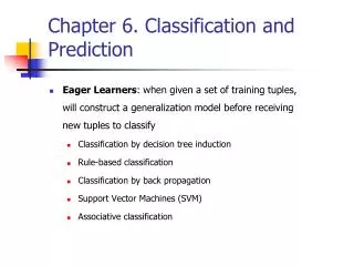
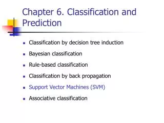
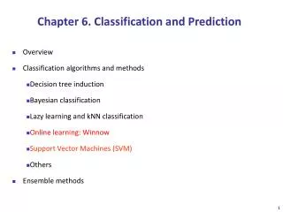
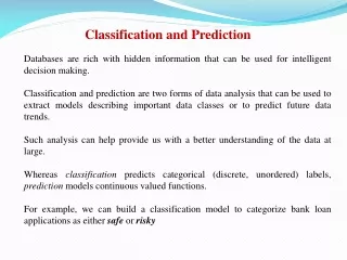
Classification by decision tree induction Bayesian classification Rule-based classification Classification by back propagation Support Vector Machines (SVM) Associative classification Chapter 6. Classification and Prediction
Bayesian Classification • A statistical classifier: performs probabilistic prediction, i.e., predicts class membership probabilities • Foundation: Based on Bayes’ Theorem. • Performance: A simple Bayesian classifier, naïve Bayesian classifier, has comparable performance with decision tree and selected neural network classifiers
Bayesian Theorem: Basics • Let X be a data sample • Let H be a hypothesis that X belongs to class C • Classification is to determine P(H|X), the probability that the hypothesis holds given the observed data sample X • Example: customer X will buy a computer given that know the customer’s age and income
Bayesian Theorem: Basics • P(H) (prior probability), the initial probability • E.g., X will buy computer, regardless of age, income, … • P(X): probability that sample data is observed • P(X|H) (posteriori probability), the probability of observing the sample X, given that the hypothesis holds • E.g.,Given that X will buy computer, the prob. that X is 31..40, medium income
Bayesian Theorem • Given training dataX, posteriori probability of a hypothesis H, P(H|X), follows the Bayes theorem
Towards Naïve Bayesian Classifier • Let D be a training set of tuples and their associated class labels, and each tuple is represented by an n-D attribute vector X = (x1, x2, …, xn) • Suppose there are m classes C1, C2, …, Cm. • Classification is to derive the maximum posteriori, i.e., the maximal P(Ci|X)
Towards Naïve Bayesian Classifier • This can be derived from Bayes’ theorem • Since P(X) is constant for all classes, only needs to be maximized
Towards Naïve Bayesian Classifier • A simplified assumption: attributes are conditionally independent (i.e., no dependence relation between attributes): • This greatly reduces the computation cost: Only counts the class distribution
Towards Naïve Bayesian Classifier • If Ak is categorical, P(xk|Ci) is the # of tuples in Ci having value xk for Ak divided by |Ci, D| (# of tuples of Ci in D) • If Ak is continous-valued, P(xk|Ci) is usually computed based on Gaussian distribution with a mean μ and standard deviation σ and P(xk|Ci) is
Naïve Bayesian Classifier: Training Dataset Class: C1:buys_computer = ‘yes’ C2:buys_computer = ‘no’ Data sample X = (age <=30, Income = medium, Student = yes Credit_rating = Fair)
Naïve Bayesian Classifier: An Example • P(Ci): P(buys_computer = “yes”) = 9/14 = 0.643 P(buys_computer = “no”) = 5/14= 0.357 • Compute P(X|Ci) for each class P(age = “<=30” | buys_computer = “yes”) = 2/9 = 0.222 P(age = “<= 30” | buys_computer = “no”) = 3/5 = 0.6 P(income = “medium” | buys_computer = “yes”) = 4/9 = 0.444 P(income = “medium” | buys_computer = “no”) = 2/5 = 0.4 P(student = “yes” | buys_computer = “yes) = 6/9 = 0.667 P(student = “yes” | buys_computer = “no”) = 1/5 = 0.2 P(credit_rating = “fair” | buys_computer = “yes”) = 6/9 = 0.667 P(credit_rating = “fair” | buys_computer = “no”) = 2/5 = 0.4
Naïve Bayesian Classifier: An Example • X = (age <= 30 , income = medium, student = yes, credit_rating = fair) P(X|Ci) : P(X|buys_computer = “yes”) = 0.222 x 0.444 x 0.667 x 0.667 = 0.044 P(X|buys_computer = “no”) = 0.6 x 0.4 x 0.2 x 0.4 = 0.019 P(X|Ci)*P(Ci) : P(X|buys_computer = “yes”) * P(buys_computer = “yes”) = 0.028 P(X|buys_computer = “no”) * P(buys_computer = “no”) = 0.007 Therefore, X belongs to class (“buys_computer = yes”)