Understanding GC Coordinate System in Theoretical Geometry
Explore the Cartesian grid and GC Coordinate System in theoretical geometry, defining space with an origin point and three axes at right angles. Learn about geometric elements like points, lines, planes, curves, and solids in relation to dimensionality.

Understanding GC Coordinate System in Theoretical Geometry
E N D
Presentation Transcript
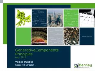
GenerativeComponents PrinciplesAug. 2010 Volker Mueller Research Director
Based on Ben Doherty’s“generative components theoretical frameworks the stuff you need to know” www.notionparallax.co.uk
Grounding in Space one fixed point in spacewith orientation etc.
Theoretical geometry gives us an infinite universe to work in. There is no concept of up, or of where we are in a finite sense. To make this work for us, we pick a spot and call it the ‘origin’.
The way of describing space that is most common is the Cartesian grid ({X,Y,Z} triples) The positive part of the Z axis can be considered ‘up’, as is the convention in building design.
Thus we have an origin (location) and 3 axes that define… 3 planes that are all at 90 degrees to each other. (The yellow line indicates the currently active plane). This is a GC- CoordinateSystem.
comfortable here? • image: Ben Doherty @ notionparallax.co.uk
…and here? • image: Ben Doherty @ notionparallax.co.uk
brilliant! • image: Ben Doherty @ notionparallax.co.uk
So, what about here? They are pretty much the same!
Almost anything can go into this box. Single values are easy to understand. Simple computations are easy, too. Scientific calculator stuff can be found in the function list. 5 Value Simple expression Function 5+2 Sin(5) fx
Almost anything can go into this box. Single values are easy to understand. Simple computations are easy, too. Scientific calculator stuff can be found in the function list. Compound statements follow BODMAS 5 Value Simple expression Function Complex expression 5+2 Sin(5) (1/Sin(5)) + 90
BODMAS B ( ) Brackets first O Orders (Powers, Roots) DM / * Division and Multiplication (left to right) AS + - Addition and Subtraction (left to right) Power: xy Pow(x,y)expl. x½ Pow(x,0.5) Root: x Sqrt(x) x Pow(x,(1/3)) 2 3
BODMAS B Brackets first O Orders (Powers, Roots) DM Division and Multiplication (left to right) AS Addition and Subtraction (left to right) 15 /(3 + 2) = ? 15 / 3 + 2 = ? (15 / 3)+ 2 = ?
BODMAS B Brackets first O Orders (Powers, Roots) DM Division and Multiplication (left to right) AS Addition and Subtraction (left to right) 15 /(3 + 2) = 3 15 / 3 + 2 = 7 (15 / 3)+ 2 = 7 IN COMPUTING, THERE ARE NEVER TOO MANY ROUND BRACKETS
Once a variable is defined (named) it can take on a value and be used in place of a value. Dave <> dave 5 dave = 8 Value Simple expression Function Complex expression Named variable Expression with named variable 5+2 Sin(5) (1/Sin(5)) + 90 dave dave*2
This circle’s radius is defined using a single value. That is how you’d expect it to work from experience. 5
This circle’s radius is defined using a list. Lists are really where the power of GC kicks in. {3,4,4.5,5}
{ , , , , , , } Type‘Curly Brackets’ { }to define a list. Things in a list are indexed from 0. Indexing uses ‘Square Brackets’ [ ] List length counts how many items are in the list, starting with 1 (here it is 5). [0] [1] [2] [3] [4]
Lists can have empty containers (null). Lists can be of different types. [0] [1] [2] [3] [4]
If we declare a variable called ‘dave’ as a list having the contents {A,B,C,D,E,F,G} Then we can refer to any item of that list individually by its index. Remember to count indices from 0. dave = {A,B,C,D,E,F,G} [0] [1] [2] [3] [4] [5] [6] dave[4] = ? dave[4] = ‘E’
Changing Dimensions …increasing and reducing geometric dimensionality
Point A point is 0 dimensional. It has no size, volume, nothing. We use a symbol for it, so that we can see it. The Point symbol is different from the CoordinateSystem symbol.
Point Its handles allow moving it using constraints. Moves can be constrained to the X,Y, and Z axes, respectively. Using the angular handles moves are constrained to the respective planes.
Line If we have 2 points, there is a line that runs through them. Strictly, lines are infinite, and line segments are bounded, but common usage refers to bounded segments as lines.
Arc, Curves …are a bit more complicated to define.
BSplineCurve The math behind splines is complicated, but the geometric description is actually quite easy. This is one of the reasons why they are used frequently.
Plane 3 points define a plane. Planes are infinite.
BSplineSurface Surfaces are in the class of 2d objects, even though they can exist in a 3d space.
Solid There are lots of ways of making solids, but they are the only truly 3d objects in GC, as they have volume. That is not to say that the rest of the things are not 3d, it is just a technical geometry distinction.
3 > 2 > 1 We can reduce dimensions, too. Solids intersected with a plane or surface produce a closed curve.
3 > 2 > 1 Surfaces intersected with a plane or surface produce an open curve (usually).
3 > 2 > 1 > 0 Curve to curve intersections produce points. Be careful of extra points! Circles and other curves are known for this problem.
3 > 2 > 1 > 0 Curve curve intersections produce points. Be careful of extra points! Circles are classic for this problem.
3 > 2 > 1 > 0 Curve curve intersections produce points. Be careful of extra points! Or no points! Circles are classic for this problem.
Almost everything we have seen so far is an object. Including input variables. In computing, objects are not equal. They have Type. dave = 8
Properties Courtesy of dot Net Framework, Microsoft
Objects have properties they can be values, or sub-objects either way, they have a type the ”dot” operator accesses an object’s properties Type some.name = “john” string some.leftLeg.foot.shoesize = 9.5 double some.rightLeg.foot.shoewidth = “wide” string some.carDrivingLicence = truebool(ean) object property dot operator
Data come in different kinds, like freight on a train. Each kind of freight requires a matching kind of freight car. Computers are similarly picky, they only deal with what they have been prepared to handle. So a type is a kind, a breed, a species, a flavor of data.
Object-oriented computing implements the idea that data and their methods, the pieces of program that manipulate these data, are bundled in packages. The general term for this is Class, i.e. a Class is a data type that includes the methods. Methods determine how objects behave. We’ll ignore for now other characteristics of OOPS.
“Simple” Variable Types (selection) bool (Boolean) Answer to a logical question (true, false) int (integer) Whole numbers (0, 5, -4, 1000, -500) double Real or decimal numbers(0.5, -7.8 ,15.0, 158.5436) string Some text (“hello world”, “450”, “dave”)
GC Classes = Feature Types (selection) Point GC’s feature type point Plane CoordinateSystem GC’s combination of point, directions, planes Direction GC’s “ray” Line Curve more general than Line, Arc, BSplineCurve BSplineSurface Solid User defined You can define your own feature types
In GC, classes are called Feature Types. For GC features the behavior is mostly generative. It is important to us how a feature gets first generated and subsequently updated. For simplicity, GC calls these methods Update Methods.