Download
1 / 31
310 likes | 329 Views
Explore new test cases for laser/accelerometer noise, differences in polar orbits, repeat modes, and the impact of various parameters on noise levels for space missions. Investigate best orbit selections for improved data accuracy.

E N D
Activities WP2420 • Mission Architecture Supervision • T. Reubelt, N. Sneeuw - GIS
New test cases • selection/discussion • new test cases for laser/accelerometer noise • new reference for laser noise • full noise vs. laser-only noise for higher orbits • SSO vs. polar orbit • repeat-mode • formations
New test cases • PSD of laser range error: • PSD of accelerometer error: • fixed parameters: ρ = 75 km, h = 350 km, I = 90°, T = 15 d
New test cases • case 2 • nfloor = 2·10-11 m/s2/sqrt(Hz) • case 3 • nfloor = 5·10-11 m/s2/sqrt(Hz) • case 1 • nrel = 5·10-13 1/sqrt(Hz) • nfloor = 1·10-11 m/s2/sqrt(Hz) • η = 3
New test cases • case 4 • nrel = (5/4)·10-13 1/sqrt(Hz) • case 5 • η = 2 • case 1 • nrel = 5·10-13 1/sqrt(Hz) • nfloor = 1·10-11 m/s2/sqrt(Hz) • η = 3
New test cases • case 6 • η = 1 • case 7 • nfloor = 5·10-11 m/s2/sqrt(Hz) • η = 2 • case 1 • nrel = 5·10-13 1/sqrt(Hz) • nfloor = 1·10-11 m/s2/sqrt(Hz) • η = 3
New test cases • Lmax = 100
New test cases • results • largest improvements by • ● reduction of white noise level (nrel) of laser • ● reduction of exponent η of the (1/f)η noise part in the low frequency range f < 0.001 Hz from η = 3 to η = 1 (or 2) • → applied in the new reference (for ρ = 75 km)
New reference for noise • PSD of laser range error: • PSD of accelerometer error: • fixed parameters: ρ = 75 km, h = 350 km, I = 90°, T = 15 d
New reference for noise • old optimistic PSD • nrel = 5·10-13 1/sqrt(Hz) • nfloor = 1·10-11 m/s2/sqrt(Hz), η = 3 • new reference • nrel = 2.67·10-13 1/sqrt(Hz) • η = 2
New reference for noise • Lmax = 100
Laser noise only for different orbit heights • total noise (laser + accelerometer) vs. laser noise only • optimistic laser PSD , ρ = 100 km, • I = 89°, T = 15 d • Lmax = 100
Laser noise only for different orbit heights • results • If accelerometer noise is regarded to be below laser noise, the degrees below l = 50 are improved (for the low orders up to 1 order of magnitude) • However, accelerometer noise can only be kept low for larger orbit heights (h > 500/600 km). This means, that the SH-errors rise rapidly for higher degrees, e.g. 1 order of magnitude for degree 50 and 2 orders of magnitude for degree 100
sun-synchronous vs. polar orbit • groundtrack-coverage at poles • polar (I = 90°) • SSO (I = 97°) • near polar (I = 93°) • repeat orbit: / = 110/7
sun-synchronous vs. polar orbit • aliasing periods for repeat orbit (/) = 110/7
sun-synchronous vs. polar orbit • aliasing periods for repeat orbit (/) = 456/29
sun-synchronous vs. polar orbit • SH/geoid-errors generated by different inclinations • polar • (I = 90°) • SSO • (I = 97°) • near polar • (I = 87°) • fixed parameters: • optimistic PSD, ρ = 100 km, • h = 300 km, T = 15 d
sun-synchronous vs. polar orbit • pros and cons of polar, near polar and sunsynchronous orbits (1) • SSO leads to a data gap of 7° • → large distortion of geoid plots around poles and of • zonal/low order SH coefficients • → such problems are almost avoided by a near polar orbit • with I = 87°/93° • SSO (and also near polar orbit) leads to a more dense and homogeneous groundtrack pattern at the areas of interest for ice studies (Greenland, Antarctic shelves); large intersection angle between ascending and descending arcs, which might improve isotropy
sun-synchronous vs. polar orbit • pros and cons of polar, near polar and sunsynchronous orbits (2) • polar orbit and SSO are problematic concerning aliasing periods of ocean tides: annual, semi-annual and very long periodic (infinite) aliasing periods occur, which might disturb signals of interest (hydrology, ice mass loss, …) • → near-polar orbits seems more suited, since such aliasing • periods are avoided • - most suited seem orbits with low inclination (e.g. TOPEX)
repeat-mode sensitivity (for hydrology and static field) new reference Lstatic≈ 200-250 → ≈ 200-500, ≈ 14-34 Lhydro≈ 70-80 → ≈ 70-160, ≈ 5-10
repeat-mode • repeat-orbit design • for hydrology an orbit with a low repeat cycle ( ≈ 70-160, ≈ 5-10) seems to be suited • problem: sensitivity for static field up to L = 200-250 • → to avoid omission errors (spatial aliasing) a solution up to L = 200-250 is needed. Thus an orbit with denser groundtrack coverage leading to a larger repeat-cycle ( ≈ 200-500, ≈ 14-34) is needed • solution? orbit with long repeat-cycle ( ≈ 30 days) for high spatial resolution and a subcycle of ≈ 7 days for temporal resolution of hydrology?
repeat-mode • What is the best option for an orbit with a repeat cycle of ≈ 30 days: • ● skipping orbit with a (pseudo-) subcycle of ≈ 7days and a homogenous gap evolution • ● skipping orbit with a distince (≈)7 day subcycle (gap evolution less homogeneous) • ● skipping orbit with a very short subcycle (semi-drifting) • ● drifting orbit
repeat-mode • skipping orbit with homogeneous gap evolution • / = 456/29, h = 333/346 km (polar/SSO), • SC = 11 days, pseudo SC = 3/11 days
repeat-mode • skipping orbit with distinct, short subcycle and • no pseudo subcycles • / = 454/29, h = 353/366 km (polar/SSO) • SC = 3 days
repeat-mode • almost drifting orbit (semi-drifting) • / = 450/29, h = 393/406 km (polar/SSO) • SC = 2 days
repeat-mode • skipping orbit with 7-day subcycle and less pronounced pseudo-subcycles • / = 467/30, h = 379/391 km (polar/SSO) • SC = 7 days, pseudo SC = 2/5 days?
repeat-mode • skipping orbit with 8-day subcycle and less pronounced pseudo-subcycles • / = 453/29, h = 363/376 km (polar/SSO) • SC = 8 days, pseudo SC = 3/5 days
formations (error propagation) fixed parameters: (/) = 219/14 (h = 357 km), σρddot = 10-10 m/s²/sqrt(Hz) PENDULUM (60/60km) GRACE (75km) CARTWHEEL (50/100km) LISA (75km)
formations (aliasing of hydrology) Echelon (GRACE) 20km / = 125/8 PENDULUM (20/10km) CARTWHEEL10/20km
formations (aliasing of hydrology) • pros and cons of formations • PENDULUM, CARTWHEEL and LISA lead to lower formal errors due to a larger isotropy and sensitivity of the sensed gravity field signal • hydrological aliasing is less for PENDULUM and larger for GRACE and CARTWHEEL • → is PENDULUM the most valuable formation?