Download
1 / 60
600 likes | 613 Views
Learn about efficient computation of data cubes, exploration in multidimensional databases, and alternative data generalization methods in data warehousing. Understand the strategies, practices, approaches, and administration involved in data warehousing development.

E N D
Data Cube Computation and Data Generation Data Warehousing資料倉儲 1001DW05 MI4 Tue.6,7(13:10-15:00)B427 Min-Yuh Day 戴敏育 Assistant Professor 專任助理教授 Dept. of Information Management, Tamkang University 淡江大學資訊管理學系 http://mail.im.tku.edu.tw/~myday/ 2011-10-11
Syllabus 週次 日期 內容(Subject/Topics) 1 100/09/06 Introduction to Data Warehousing 2 100/09/13 Data Warehousing, Data Mining, and Business Intelligence 3 100/09/20 Data Preprocessing: Integration and the ETL process 4 100/09/27 Data Warehouse and OLAP Technology 5 100/10/04 Data Warehouse and OLAP Technology 6 100/10/11 Data Cube Computation and Data Generation 7 100/10/18 Data Cube Computation and Data Generation 8 100/10/25 Project Proposal 9 100/11/01 期中考試週
Syllabus 週次 日期 內容(Subject/Topics) 10 100/11/08 Association Analysis 11 100/11/15 Classification and Prediction 12 100/11/22 Cluster Analysis 13 100/11/29 Sequence Data Mining 14 100/12/06 Social Network Analysis 15 100/12/13 Link Mining 16 100/12/20 Text Mining and Web Mining 17 100/12/27 Project Presentation 18 101/01/03 期末考試週
Data Warehouse Development • Data warehouse development approaches • Inmon Model: EDW approach (top-down) • Kimball Model: Data mart approach (bottom-up) • Which model is best? • There is no one-size-fits-all strategy to DW • One alternative is the hosted warehouse • Data warehouse structure: • The Star Schema vs. Relational • Real-time data warehousing? Source: Turban et al. (2011), Decision Support and Business Intelligence Systems
DW Development Approaches (Kimball Approach) (Inmon Approach) Source: Turban et al. (2011), Decision Support and Business Intelligence Systems
DW Structure: Star Schema(a.k.a. Dimensional Modeling) Source: Turban et al. (2011), Decision Support and Business Intelligence Systems
Dimensional Modeling • Data cube • A two-dimensional, three-dimensional, or higher-dimensional object in which each dimension of the data represents a measureof interest • Grain • Drill-down • Slicing Source: Turban et al. (2011), Decision Support and Business Intelligence Systems
Best Practices for Implementing DW The project must fit with corporate strategy There must be complete buy-in to the project It is important to manage user expectations The data warehouse must be built incrementally Adaptability must be built in from the start The project must be managed by both IT and business professionals (a business–supplier relationship must be developed) Only load data that have been cleansed/high quality Do not overlook training requirements Be politically aware. Source: Turban et al. (2011), Decision Support and Business Intelligence Systems
Real-time DW(a.k.a. Active Data Warehousing) • Enabling real-time data updates for real-time analysis and real-time decision making is growing rapidly • Push vs. Pull (of data) • Concerns about real-time BI • Not all data should be updated continuously • Mismatch of reports generated minutes apart • May be cost prohibitive • May also be infeasible Source: Turban et al. (2011), Decision Support and Business Intelligence Systems
Evolution of DSS & DW Source: Turban et al. (2011), Decision Support and Business Intelligence Systems
Active Data Warehousing (by Teradata Corporation) Source: Turban et al. (2011), Decision Support and Business Intelligence Systems
Comparing Traditional and Active DW Source: Turban et al. (2011), Decision Support and Business Intelligence Systems
Data Warehouse Administration • Due to its huge size and its intrinsic nature, a DW requires especially strong monitoring in order to sustain its efficiency, productivity and security. • The successful administration and management of a data warehouse entails skills and proficiency that go past what is required of a traditional database administrator. • Requires expertise in high-performance software, hardware, and networking technologies Source: Turban et al. (2011), Decision Support and Business Intelligence Systems
Data Cube Computation and Data Generalization • Efficient Computation of Data Cubes • Exploration and Discovery in Multidimensional Databases • Attribute-Oriented Induction ─ An Alternative Data Generalization Method Source: Han & Kamber (2006)
Efficient Computation of Data Cubes • Preliminary cube computation tricks • Computing full/iceberg cubes: 3 methodologies • Top-Down: Multi-Way array aggregation • Bottom-Up: • Bottom-up computation: BUC • H-cubing technique • Integrating Top-Down and Bottom-Up: • Star-cubing algorithm • High-dimensional OLAP: A Minimal Cubing Approach • Computing alternative kinds of cubes: • Partial cube, closed cube, approximate cube, etc. Source: Han & Kamber (2006)
Preliminary Tricks (Agarwal et al. VLDB’96) • Sorting, hashing, and grouping operations are applied to the dimension attributes in order to reorder and cluster related tuples • Aggregates may be computed from previously computed aggregates, rather than from the base fact table • Smallest-child: computing a cuboid from the smallest, previously computed cuboid • Cache-results: caching results of a cuboid from which other cuboids are computed to reduce disk I/Os • Amortize-scans: computing as many as possible cuboids at the same time to amortize disk reads • Share-sorts: sharing sorting costs cross multiple cuboids when sort-based method is used • Share-partitions: sharing the partitioning cost across multiple cuboids when hash-based algorithms are used Source: Han & Kamber (2006)
Multi-Way Array Aggregation • Array-based “bottom-up” algorithm • Using multi-dimensional chunks • No direct tuple comparisons • Simultaneous aggregation on multiple dimensions • Intermediate aggregate values are re-used for computing ancestor cuboids • Cannot do Apriori pruning: No iceberg optimization Source: Han & Kamber (2006)
C c3 61 62 63 64 c2 45 46 47 48 c1 29 30 31 32 c 0 B 60 13 14 15 16 b3 44 28 56 9 b2 B 40 24 52 5 b1 36 20 1 2 3 4 b0 a0 a1 a2 a3 A Multi-way Array Aggregation for Cube Computation (MOLAP) • Partition arrays into chunks (a small subcube which fits in memory). • Compressed sparse array addressing: (chunk_id, offset) • Compute aggregates in “multiway” by visiting cube cells in the order which minimizes the # of times to visit each cell, and reduces memory access and storage cost. What is the best traversing order to do multi-way aggregation? Source: Han & Kamber (2006)
C c3 61 62 63 64 c2 45 46 47 48 c1 29 30 31 32 c 0 B 60 13 14 15 16 b3 44 28 56 9 b2 40 24 52 5 b1 36 20 1 2 3 4 b0 a0 a1 a2 a3 A Multi-way Array Aggregation for Cube Computation B Source: Han & Kamber (2006)
Multi-way Array Aggregation for Cube Computation C c3 61 62 63 64 c2 45 46 47 48 c1 29 30 31 32 c 0 B 60 13 14 15 16 b3 44 28 B 56 9 b2 40 24 52 5 b1 36 20 1 2 3 4 b0 a0 a1 a2 a3 A Source: Han & Kamber (2006)
Multi-Way Array Aggregation for Cube Computation (Cont.) • Method: the planes should be sorted and computed according to their size in ascending order • Idea: keep the smallest plane in the main memory, fetch and compute only one chunk at a time for the largest plane • Limitation of the method: computing well only for a small number of dimensions • If there are a large number of dimensions, “top-down” computation and iceberg cube computation methods can be explored Source: Han & Kamber (2006)
Bottom-Up Computation (BUC) • BUC (Beyer & Ramakrishnan, SIGMOD’99) • Bottom-up cube computation (Note: top-down in our view!) • Divides dimensions into partitions and facilitates iceberg pruning • If a partition does not satisfy min_sup, its descendants can be pruned • If minsup = 1 Þ compute full CUBE! • No simultaneous aggregation Source: Han & Kamber (2006)
BUC: Partitioning • Usually, entire data set can’t fit in main memory • Sort distinct values, partition into blocks that fit • Continue processing • Optimizations • Partitioning • External Sorting, Hashing, Counting Sort • Ordering dimensions to encourage pruning • Cardinality, Skew, Correlation • Collapsing duplicates • Can’t do holistic aggregates anymore! Source: Han & Kamber (2006)
Star-Cubing: An Integrating Method • Integrate the top-down and bottom-up methods • Explore shared dimensions • E.g., dimension A is the shared dimension of ACD and AD • ABD/AB means cuboid ABD has shared dimensions AB • Allows for shared computations • e.g., cuboid AB is computed simultaneously as ABD • Aggregate in a top-down manner but with the bottom-up sub-layer underneath which will allow Apriori pruning • Shared dimensions grow in bottom-up fashion Source: Han & Kamber (2006)
Iceberg Pruning in Shared Dimensions • Anti-monotonic property of shared dimensions • If the measure is anti-monotonic, and if the aggregate value on a shared dimension does not satisfy the iceberg condition, then all the cells extended from this shared dimension cannot satisfy the condition either • Intuition: if we can compute the shared dimensions before the actual cuboid, we can use them to do Apriori pruning • Problem: how to prune while still aggregate simultaneously on multiple dimensions? Source: Han & Kamber (2006)
Cell Trees • Use a tree structure similar to H-tree to represent cuboids • Collapses common prefixes to save memory • Keep count at node • Traverse the tree to retrieve a particular tuple Source: Han & Kamber (2006)
Star Attributes and Star Nodes • Intuition: If a single-dimensional aggregate on an attribute value p does not satisfy the iceberg condition, it is useless to distinguish them during the iceberg computation • E.g., b2, b3, b4, c1, c2, c4, d1, d2, d3 • Solution: Replace such attributes by a *. Such attributes are star attributes, and the corresponding nodes in the cell tree are star nodes Source: Han & Kamber (2006)
Example: Star Reduction • Suppose minsup = 2 • Perform one-dimensional aggregation. Replace attribute values whose count < 2 with *. And collapse all *’s together • Resulting table has all such attributes replaced with the star-attribute • With regards to the iceberg computation, this new table is a loseless compression of the original table Source: Han & Kamber (2006)
Efficient Computation of Data Cubes • Exploration and Discovery in Multidimensional Databases • Attribute-Oriented Induction ─ An Alternative Data Generalization Method Source: Han & Kamber (2006)
Computing Cubes with Non-Antimonotonic Iceberg Conditions • Most cubing algorithms cannot compute cubes with non-antimonotonic iceberg conditions efficiently • Example CREATE CUBE Sales_Iceberg AS SELECT month, city, cust_grp, AVG(price), COUNT(*) FROM Sales_Infor CUBEBY month, city, cust_grp HAVINGAVG(price) >= 800 AND COUNT(*) >= 50 • Needs to study how to push constraint into the cubing process Source: Han & Kamber (2006)
Non-Anti-Monotonic Iceberg Condition • Anti-monotonic: if a process fails a condition, continue processing will still fail • The cubing query with avg is non-anti-monotonic! • (Mar, *, *, 600, 1800) fails the HAVING clause • (Mar, *, Bus, 1300, 360) passes the clause CREATE CUBE Sales_Iceberg AS SELECT month, city, cust_grp, AVG(price), COUNT(*) FROM Sales_Infor CUBEBY month, city, cust_grp HAVING AVG(price) >= 800AND COUNT(*) >= 50 Source: Han & Kamber (2006)
From Average to Top-k Average • Let (*, Van, *) cover 1,000 records • Avg(price) is the average price of those 1000 sales • Avg50(price) is the average price of the top-50 sales (top-50 according to the sales price • Top-k average is anti-monotonic • The top 50 sales in Van. is with avg(price) <= 800 the top 50 deals in Van. during Feb. must be with avg(price) <= 800 Source: Han & Kamber (2006)
Binning for Top-k Average • Computing top-k avg is costly with large k • Binning idea • Avg50(c) >= 800 • Large value collapsing: use a sum and a count to summarize records with measure >= 800 • If count>=800, no need to check “small” records • Small value binning: a group of bins • One bin covers a range, e.g., 600~800, 400~600, etc. • Register a sum and a count for each bin Source: Han & Kamber (2006)
Computing Approximate top-k average Suppose for (*, Van, *), we have Approximate avg50()= (28000+10600+600*15)/50=952 Top 50 The cell may pass the HAVING clause Source: Han & Kamber (2006)
Weakened Conditions Facilitate Pushing • Accumulate quant-info for cells to compute average iceberg cubes efficiently • Three pieces: sum, count, top-k bins • Use top-k bins to estimate/prune descendants • Use sum and count to consolidate current cell weakest strongest Source: Han & Kamber (2006)
Computing Iceberg Cubes with Other Complex Measures • Computing other complex measures • Key point: find a function which is weaker but ensures certain anti-monotonicity • Examples • Avg() v: avgk(c) v (bottom-k avg) • Avg() v only (no count): max(price) v • Sum(profit) (profit can be negative): • p_sum(c) v if p_count(c) k; or otherwise, sumk(c) v • Others: conjunctions of multiple conditions Source: Han & Kamber (2006)
Efficient Computation of Data Cubes • Exploration and Discovery in Multidimensional Databases • Attribute-Oriented Induction ─ An Alternative Data Generalization Method Source: Han & Kamber (2006)
Discovery-Driven Exploration of Data Cubes • Hypothesis-driven • exploration by user, huge search space • Discovery-driven (Sarawagi, et al.’98) • Effective navigation of large OLAP data cubes • pre-compute measures indicating exceptions, guide user in the data analysis, at all levels of aggregation • Exception: significantly different from the value anticipated, based on a statistical model • Visual cues such as background color are used to reflect the degree of exception of each cell Source: Han & Kamber (2006)
Kinds of Exceptions and their Computation • Parameters • SelfExp: surprise of cell relative to other cells at same level of aggregation • InExp: surprise beneath the cell • PathExp: surprise beneath cell for each drill-down path • Computation of exception indicator (modeling fitting and computing SelfExp, InExp, and PathExp values) can be overlapped with cube construction • Exception themselves can be stored, indexed and retrieved like precomputed aggregates Source: Han & Kamber (2006)
Examples: Discovery-Driven Data Cubes Source: Han & Kamber (2006)
Complex Aggregation at Multiple Granularities: Multi-Feature Cubes • Multi-feature cubes (Ross, et al. 1998): Compute complex queries involving multiple dependent aggregates at multiple granularities • Ex. Grouping by all subsets of {item, region, month}, find the maximum price in 1997 for each group, and the total sales among all maximum price tuples select item, region, month, max(price), sum(R.sales) from purchases where year = 1997 cube by item, region, month: R such that R.price = max(price) • Continuing the last example, among the max price tuples, find the min and max shelf live, and find the fraction of the total sales due to tuple that have min shelf life within the set of all max price tuples Source: Han & Kamber (2006)
Cube-Gradient (Cubegrade) • Analysis of changes of sophisticated measures in multi-dimensional spaces • Query: changes of average house price in Vancouver in ‘00 comparing against ’99 • Answer: Apts in West went down 20%, houses in Metrotown went up 10% • Cubegrade problem by Imielinski et al. • Changes in dimensions changes in measures • Drill-down, roll-up, and mutation Source: Han & Kamber (2006)
From Cubegrade to Multi-dimensional Constrained Gradients in Data Cubes • Significantly more expressive than association rules • Capture trends in user-specified measures • Serious challenges • Many trivial cells in a cube “significance constraint” to prune trivial cells • Numerate pairs of cells “probe constraint” to select a subset of cells to examine • Only interesting changes wanted “gradient constraint” to capture significant changes Source: Han & Kamber (2006)
MD Constrained Gradient Mining • Significance constraint Csig: (cnt100) • Probe constraint Cprb: (city=“Van”, cust_grp=“busi”, prod_grp=“*”) • Gradient constraint Cgrad(cg, cp): (avg_price(cg)/avg_price(cp)1.3) (c4, c2) satisfies Cgrad! Probe cell: satisfied Cprb Base cell Aggregated cell Siblings Ancestor Source: Han & Kamber (2006)
Efficient Computing Cube-gradients • Compute probe cells using Csig and Cprb • The set of probe cells P is often very small • Use probe P and constraints to find gradients • Pushing selection deeply • Set-oriented processing for probe cells • Iceberg growing from low to high dimensionalities • Dynamic pruning probe cells during growth • Incorporating efficient iceberg cubing method Source: Han & Kamber (2006)
Efficient Computation of Data Cubes • Exploration and Discovery in Multidimensional Databases • Attribute-Oriented Induction ─ An Alternative Data Generalization Method Source: Han & Kamber (2006)
Data Generalization and Summarization-based Characterization • Data generalization • A process which abstracts a large set of task-relevant data in a database from a low conceptual levels to higher ones. • Approaches: • Data cube approach(OLAP approach) • Attribute-oriented induction approach 1 Higher level: Young, Old 2 3 4 Lower level: 18 , 70 in Age Conceptual levels 5 Source: Han & Kamber (2006)
What is Concept Description? • Descriptive vs. predictive data mining • Descriptive mining: describes concepts or task-relevant data sets in concise, summarative, informative, discriminative forms • Predictive mining: Based on data and analysis, constructs models for the database, and predicts the trend and properties of unknown data • Concept description: • Characterization: provides a concise and succinct summarization of the given collection of data • Comparison: provides descriptions comparing two or more collections of data Source: Han & Kamber (2006)
Concept Description vs. OLAP • Similarity: • Data generalization • Presentation of data summarization at multiple levels of abstraction. • Interactivedrilling, pivoting, slicing and dicing. • Differences: • Can handle complex data types of the attributes and their aggregations • Automated desired level allocation. • Dimension relevance analysis and ranking when there are many relevant dimensions. • Sophisticated typing on dimensions and measures. • Analytical characterization: data dispersion analysis Source: Han & Kamber (2006)
Attribute-Oriented Induction • Collect the task-relevant data (initial relation) using a relational database query • Perform generalization by attribute removal or attribute generalization • Apply aggregation by merging identical, generalized tuples and accumulating their respective counts • Interactive presentation with users Source: Han & Kamber (2006)