Download

1 / 21
210 likes | 356 Views
Power Variation Strategies in Cycling Time Trials. Louis Grisez. Overview. Abstract Introducing Cycling Creation of a Mathematical Model Initial Conditions Calibration Results. Abstract . The ultimate goal of cycling time trials Need for a pacing strategy Energy Depletion

E N D
Power Variation Strategies in Cycling Time Trials Louis Grisez
Overview • Abstract • Introducing Cycling • Creation of a Mathematical Model • Initial Conditions • Calibration • Results
Abstract • The ultimate goal of cycling time trials • Need for a pacing strategy • Energy Depletion • Mean work rate and various pacing strategies. • This research is a verification of the steady state approximation used in "Power variation strategies for cycling time trials: A differential equation model" by author, Graeme P.Boswell • Seeks to improve the optimal pacing strategy found previously using a steady-state approximation. • Energy based differential equation • Model will be used in theoretical courses with varying conditions and cyclists of different masses.
An Introduction to Cycling • Competitive event rode in the fastest way possible • National, world, and Olympic championship events • Races are a primarily measurement of athletic ability over a period of time. • Only known tactic: • Suggested method: uniform work output rate • Assumption: constant conditions of power output as well as resistive forces • Refined method: Altered power output • Models altering course conditions such as road gradient • This is done as an improved method compared to the steady state approximation in reducing the time needed to complete the course. • Previous studies (Gordon, 2005; Swain 1997) have shown the validity of variable power output approximations.
The Steady State • Accelerations are assumed to be instantaneous (Swain 1997). • Considered being in steady state • Showed that the refined method had a time saving effect as high as 8.3 percent compared to the constant work rate. • This actually increased with the growing incline of the track. • Problem concerning these assumptions • instantaneous acceleration: do not directly apply to road cycling • This problem was later improved by Atkinson's improved calibration model. • Kinetic energy and speed were observed at one second intervals. • Jumps in velocity were approximated as continuous acceleration. • changes in velocity between the transitions were ignored • The variable pacing strategy used by both Swain and Atkinson increased the mean power beyond the constant power approximation by as high as 10 percent due to the ascending time being greater than the descending time. As a burden, this pacing strategy may be overestimated.
Mathematical Model • Cyclist must apply power to the drive chain. • The combined speed of the bicycle is a function of the difference between P and Δ • P is applied power • Δ is power of resistive forces • Three Resistive forces • Gravity • Rolling • Wind
Mathematical Model • Rate of change of kinetic energy
Mathematical Model • Assuming there are no changes in the rider's velocity due to varying grades, surfaces, wind strength and applied power, the previous equation becomes • This is the steady state
Initial Conditions • Initial data points, given by G. Boswell to be: • x(0)=0 • v(0)=0 • Initial data points used • v(0)=1 • Small enough to be negligible in terms of final output. • This is also the first instance in which procedure differed from that of previous work done by G. Boswell. • Assuming there are no changes in the rider's velocity due to varying grades, surfaces, wind strength and applied power, equation $(5)$ can be written as
Calibration • Constants need to be defined • Assumption: • Rider does not refer to tuck position • Cyclists were pulled behind vehicles • Eliminates the variability of power output and small changes in velocity • Human Athletic Performance
Human Athletic Performance • Oxygen limitation • Events last 2-3 hours • Average oxygen intake of 3.7 • (Swain,1997) • Human biomechanical performance • 25% efficient
Courses • 10 [km] flat • 5 [km] uphill followed by 5 [km] downhill • Alternating 1 [km] sections • Alternating 0.5 [km] sections • Variable gradients of: 5, 10, 15% • Variable power of: 5, 10, 15%
Pacing Strategies • Research separates from G. Boswell • Initial: • Increase of power as a percent • Decrease using • Final: • Increase of power as a percent • Decrease of power as same percent
Solution Methods • Use of MATLAB 2012 • Numerical Solver ode45 • Set of 4 integrated for loops
Results of Change in KE • Compared to data found by G. Boswell • 2% error • Less time for cyclist to complete course
Progress on Steady State • Use of ode solver to model the original steady state approximation • Function is to create comparable data to variable pacing strategy • Results show a very high error • MATLAB solver error • Possible benefits • Time saving could be potentially over 10%
Conclusion • Cycling as a whole • Relevance of a pacing strategy • Results • Future Improvements
Hickethier, D. (2013). Personal interview Di Prampero, P.E., Cortelli, G. Mognomi, P., & Saibene, F. (1979). Equation of motion of a cyclist. Journal of Applied Physiology, 47, 201-206. Gordon, S (2005). Optimizing distribution of power during a cycling time trial. Sports Engineering, 8, 81-90. Graeme P. Boswell (2012): Power variation strategies for cycling time trials: A differential equation model, Journal of Sports Sciences, 30:7, 651-659. Martin, J. C., Gardner, A. S., Barras, M., & Martin, D. T. (2006) Modelling sprint cycling using field-derived parameters and forward integration. Medicine and Science in Sports and Exercise, 3, 592-597.