Download
1 / 59
590 likes | 769 Views
Strategies for handling missing data in randomised trials. Peninsula Medical School, Exeter, 14 th March 2011 Ian White, MRC Biostatistics Unit, Cambridge, UK. Plan. Why do missing data matter? Intention-to-treat analysis strategy for randomised trials with missing outcomes

E N D
Strategies for handling missing data in randomised trials Peninsula Medical School, Exeter, 14th March 2011 Ian White, MRC Biostatistics Unit, Cambridge, UK
Plan • Why do missing data matter? • Intention-to-treat analysis strategy for randomised trials with missing outcomes • Analysis methods • regression and mixed models • Sensitivity analysis • methods & examples • Missing baseline covariates • simple methods are best • Please ask questions! • Work with: James Carpenter & Stuart Pocock (LSHTM), Nick Horton (USA), Simon Thompson (BSU)
Why do missing data matter? • Loss of power (cf. power with no missing data) • can’t regain lost power • Any analysis must make an untestable assumption about the missing data • wrong assumption biased estimates • Some popular analyses with missing data get biased standard errors • resulting in wrong p-values and confidence intervals • Some popular analyses with missing data are inefficient • confidence intervals wider than they need be
What to do: loss of power Can’t solve by analysis (but can exacerbate it!). Approach by design: • Minimise amount of missing data • Good communications with participants • Aim to follow everyone up • Make repeated attempts using different methods • Also good to reduce the impact of missing data • Collect reasons for missing data • Collect information predictive of missing values • Now assume that despite doing our best we still have some missing data…
What to do: analysis A suitable method of analysis would: • Make the correct assumption about the missing data • Give an unbiased estimate (under that assumption) • Give an unbiased standard error (so that P-values and confidence intervals are correct) • Be efficient (make best use of the available data) we can never be sure what is the correct assumptionsensitivity analyses are essential
Loss of power Bias Outcome Exposure Confounders Fail to control confounding Potentially inefficient analysis Missing data problems: observational studies
Loss of power Bias Outcome Baseline covariates Exposure Confounders Randomised group Fail to control confounding Potentially inefficient analysis Missing data problems: randomised trials
Plan • Why do missing data matter? • Intention-to-treat analysis strategy for randomised trials with missing outcomes • Analysis methods • regression and mixed models • Sensitivity analysis • methods & examples • Missing baseline covariates • simple methods are best
Intention-to-treat (ITT) principle • The ITT principle says that we should: • include everyone randomised • in the group to which they were assigned (whether or not they completed the intervention given to the group) • With missing data, this is easier said than done • I’m going to show it can also conflict with the statistical principle that the analysis should be valid under plausible assumptions
Note • I’m addressing the ITT hypothesis • “There is no difference in clinical outcome between these two randomised groups” • & estimating the ITT difference • difference in clinical outcome between randomised groups
What does intention-to-treat mean when some outcome data are missing? (1) • A strict view is that ITT requires complete outcome data • but researchers with incomplete outcome data also need a principle to guide them • Should all randomised individuals still be included? • “Although those participants [who drop out] cannot be included in the analysis, it is customary still to refer to analysis of all available participants as an intention-to-treat analysis” (Altman et al, 2001) • “Complete case analysis, which was the approach used in most trials, violates the principle of intention to treat” (Hollis & Campbell, 1999)
What does intention-to-treat mean when some outcome data are missing? (2) • In new advice, the European Medicines Agency (2010) takes a more relaxed view: • “Full set analysis generally requires the imputation of values or modelling for the unrecorded data” • The CONSORT (2010) statement says: • “We replaced mention of ‘intention to treat’ analysis, a widely misused term, by a more explicit request for information about retaining participants in their original assigned groups”
Difficulties • Including all randomised individuals in the analysis isn’t enough to make an analysis valid • The desire to include all randomised individuals in the analysis • reduces emphasis on the appropriate assumptions • leads to uncritical use of simple imputation methods, esp. Last Observation Carried Forward (LOCF) • leads to unnecessary use of complex methods, esp. multiple imputation • I’m going to say a bit about LOCF, then explain how we have re-defined ITT as an analysis strategy
80 60 Y 40 20 0 0 3 6 9 12 Months Last observation carried forward (LOCF)
LOCF: why it is used • LOCF is widely advocated • e.g. the European drugs regulator wrote (CPMP 2001, but since revised): • “The statistical analysis of a clinical trial generally requires the imputation of values to those data that have not been recorded …” • “Last observation carried forward … is likely to be acceptable if measurements are expected to be relatively constant over time.”
LOCF: what it assumes • Assumes last observation is representative of the missing value • Can’t verify this assumption from the data • e.g. even if there was no observed trend over time, drop-outs could have deteriorated • Analysts rarely give a good justification, and instead justify LOCF (wrongly) on the grounds that • it is conservative: not true in general • it respects ITT by analysing all individuals • LOCF widely critiqued e.g. Mallinckrodt et al (2004) • Should only be used if its assumption is plausible! • So how can we unlink ITT from methods like LOCF?
Strategy for intention to treat analysis with incomplete observations (White et al, BMJ, 2011) • Attempt to follow up all randomised participants, even if they withdraw from allocated treatment • Perform a main analysis of all observed data that is valid under a plausible assumption about the missing data • Perform sensitivity analyses to explore the effect of departures from the assumption made in the main analysis • Account for all randomised participants, at least in the sensitivity analyses
Example 1: QUATRO trial European multicentre RCT to evaluate the effectiveness of adherence therapy in improving quality of life for people with schizophrenia (Gray et al, 2006) Primary outcome: quality of life measured by the SF-36 MCS scale, measured at baseline and 52-week follow up 18
QUATRO trial: analyses • We did attempt to follow up all randomised individuals • Main assumption: no difference between missing and observed values, once adjusted for baseline variables (MAR) • Main analysis: analysis of covariance on complete cases • intervention effect = -0.33 (s.e. 1.11) • Sensitivity analysis: consider possible differences between missing and observed values, allowed to be different in each arm • see later
observed data M missing data Missing at random (MAR) • The probability that data are missing depends on the values of the observed data, but does not depend on the values of the missing data • p(M | Yobs, Ymis) = p(M | Yobs)
Plan • Why do missing data matter? • Intention-to-treat analysis strategy for randomised trials with missing outcomes • Analysis methods • regression and mixed models • Sensitivity analysis • methods & examples • Missing baseline covariates • simple methods are best
How to approach the analysis • Principled approach to missing data: • start by identifying a plausible assumption • then choose an analysis method that’s valid under that assumption • Some analysis methods are simple to describe but have complex assumptions
The analysis toolkit Simple methods • Last observation carried forward (LOCF) • Complete-case analysis • Mean imputation • Missing indicator method • Regression imputation More complex methods • Multiple imputation • Likelihood-based methods • Inverse probability weighting (IPW)
Properties of methods Valid means valid & efficient
A comment on MAR • A lot of statistical literature seems to regard MAR as the correct starting point for analyses with missing data • One argument in favour of MAR is that it tends to become more plausible as more variables are included in the model • unlike other assumptions • I think the correct assumption depends on the clinical context • However in this section I’m going to assume MAR
What method is best for missing outcomes in a RCT, assuming MAR? With a single outcome (not repeated measures): • Regress outcome (Y) on randomised group (Z), adjusting for baseline covariates (X) • analysis of covariance, ANCOVA • this is the likelihood-based method • Which X? • to make MAR valid, adjust for X that predict both outcome and missingness • to gain power, adjust for X that predict outcome • Cases with missing Y contribute no information • complete-cases analysis is correct!
What method is best for missing outcomes in a RCT, assuming MAR? With a repeated outcome: • Use a mixed model (likelihood-based) • Include all observed outcome data • Exclude any individuals with no post-baseline observations • Include X’s as before Software: • Stata xtmixed, SAS proc mixed, R lme() Some points to note: • Don’t allow a treatment effect at baseline • Allow a different treatment effect at each follow-up time • If possible, allow for correlations between outcomes via an unstructured variance-covariance matrix
What about multiple imputation? Idea of multiple imputation: • Impute missing (single or longitudinal) outcomes from observed outcomes and baselines repeat m times • Analyse the m completed data sets • Combine estimates by Rubin’s rules Tutorial: White et al (2011)
Multiple imputation and ITT • MI includes all randomised individuals in the analysis • appealing • Example with single outcome (Riper et al, 2008): • “We then performed intention-to-treat analysis, using multiple imputation to deal with loss to follow-up.” • MI is the same as fitting a [mixed] model to the observed data if imputation model and analysis model are the same • but MI has additional random error (“Monte Carlo error”) due to using a finite number of imputed data sets • so why do MI? • MI may be of value in a RCT • if additional information (“auxiliary variables”, e.g. compliance) can be included in the imputation model • as a way to do sensitivity analyses
0.01 0.004 Example: UK700 trial • Intensive vs. Standard case management for severely mentally ill people living in the community • 708 patients randomised in 4 UK centres • Outcome here: CPRS (psychopathology) score from 2-year interview (missing in 11% of Intensive, 20% of Standard) Monte Carlo error
Plan • Why do missing data matter? • Intention-to-treat analysis strategy for randomised trials with missing outcomes • Analysis methods • regression and mixed models • Sensitivity analysis • methods & examples • Missing baseline covariates • simple methods are best
CC MAR-based 10 9 Mean outcome 8 7 6 0 1 2 0 1 2 0 1 2 time Complete Drop out at time 1 How to do sensitivity analyses? • Not LOCF for main analysis, CC for sensitivity analysis LOCF
Principled sensitivity analysis • Not LOCF for main analysis, CC for sensitivity analysis • the alternative assumptions should contradict the main assumption • Instead, specify the numerical value of “sensitivity parameter(s)” governing the degree of departure from the main assumption (Kenward et al, 2001) • e.g. the degree of departure from MAR • Want methods to exactly match the main analysis when sensitivity parameter is zero • I’ll first describe methods based around an MAR-based main analysis, then go further
Mean score approach (1) • Analysis model: E[Y|X] = h(bAX) • Y is outcome • h(.) is inverse link function (e.g. identity or invlogit) • X is a covariate vector including 1's, randomised group Z and baseline covariates – we're interested in the component of bA corresponding to Z • Missing data occur in Y only • MY is missingness of Y
Mean score approach (2) • Analysis model: E[Y|X] = h(bAX) • Imputation model: E[Y|X,MY] = h(bIX + MYd) • dis a user-specified departure from MAR: could be d1 if randomised to arm 1, d0if randomised to arm 0. • Estimate bI by regressing Y on X in complete cases (MY=0) • If we had complete data we would estimate the analysis model using estimating equations S X{Y - h(bAX)} = 0 • Replace missing Y with Y* = E[Y|X,MY=1] = h(bIX + d) • Solve! • Standard errors by sandwich method (based on EEs for both bI and bA) or by conditional variance formula • Simplifies in the special case of linear regression
MAR Example: QUATRO data Outcome SD ≈ 12
Why do I allow different missing data mechanisms in different arms? • Because data may be further from MAR after more intensive interventions • Because results are most sensitive to this
Simple approach • Assumed departures from MAR: • let d = mean unobserved – mean observed outcome • taking values d0 , d1 in arm 0, 1 • Values estimated from observed data: • p0, p1 = fraction of missing data in arm 0, 1 • DCC = intervention effect in complete cases • D = true intervention effect • Then we can show (White et al, 2007) that • D = DCC + d1p1 – d0p0 • se(D) ≈ se(DCC) • Back-of-an-envelope calculation!
1.13 1.12 1.11 estimated intervention effect Standard error of 1.1 1.09 -10 -8 -6 -4 -2 0 d = Missing – Observed Intervention only Both arms Control only Are std errors affected by d? (QUATRO)
Alternatives to mean score approach • Can use MI • Define imputation and analysis models as before • Fit imputation model to complete cases as before • Impute with offset d • implemented in ice • For sensitivity analysis, best to use same seed across different values of d • Can use IPW • involves specifying d in missingness model logit P(MY=1|Y,X) = aX + dY
Demonstration using rctmiss in Stata Missing data are 5 units (0.5 SD) worse than observed: . rctmiss, pmmdelta(-5): reg sf_mcs alloc sf_mcsba …in both arms MNAR regression results ------------------------------------------------------------------------------ sf_mcs | Coef. Std. Err. z P>|z| [95% Conf. Interval] -------------+---------------------------------------------------------------- alloc | -.7338669 1.096779 -0.67 0.503 -2.883514 1.415781 sf_mcsba | .4697194 .0497254 9.45 0.000 .3722594 .5671794 _cons | 22.37387 2.058745 10.87 0.000 18.33881 26.40894 ------------------------------------------------------------------------------ . rctmiss, pmmdelta(cond(alloc,-5,0)): reg sf_mcs alloc sf_mcsba … in intervention arm only MNAR regression results ------------------------------------------------------------------------------ sf_mcs | Coef. Std. Err. z P>|z| [95% Conf. Interval] -------------+---------------------------------------------------------------- alloc | -1.016182 1.093445 -0.93 0.353 -3.159295 1.126931 sf_mcsba | .4695661 .0496591 9.46 0.000 .372236 .5668962 _cons | 22.66207 2.052232 11.04 0.000 18.63977 26.68437 ------------------------------------------------------------------------------ rctmiss also produces the graph
Corespondence with MAR when D=0 . reg sf_mcs alloc sf_mcsba Standard MAR analysis Source | SS df MS Number of obs = 349 -------------+------------------------------ F( 2, 346) = 49.42 Model | 10497.5347 2 5248.76733 Prob > F = 0.0000 Residual | 36748.2816 346 106.208906 R-squared = 0.2222 -------------+------------------------------ Adj R-squared = 0.2177 Total | 47245.8162 348 135.76384 Root MSE = 10.306 ------------------------------------------------------------------------------ sf_mcs | Coef. Std. Err. t P>|t| [95% Conf. Interval] -------------+---------------------------------------------------------------- alloc | -.3341637 1.108198 -0.30 0.763 -2.513817 1.84549 sf_mcsba | .4703734 .0475847 9.88 0.000 .3767818 .5639651 _cons | 22.62969 2.05461 11.01 0.000 18.5886 26.67079 ------------------------------------------------------------------------------ . rctmiss, pmmdelta(0): reg sf_mcs alloc sf_mcsba Results allowing for MNAR Using 349 complete cases and 37 incomplete cases ------------------------------------------------------------------------------ sf_mcs | Coef. Std. Err. z P>|z| [95% Conf. Interval] -------------+---------------------------------------------------------------- alloc | -.3341637 1.108198 -0.30 0.763 -2.506193 1.837865 sf_mcsba | .4703734 .0475847 9.88 0.000 .3771091 .5636377 _cons | 22.62969 2.05461 11.01 0.000 18.60273 26.65665 ------------------------------------------------------------------------------
Main difficulty • How to specify d? • Need to discuss with investigators • aim to pre-specify • Alternatively report value of d that changes [significance of] conclusions
Example 2: smoking cessation trial • Smokers calling a telephone helpline were randomised to tailored advice letters + standard counselling or standard counselling • Sutton & Gilbert (2007) • Outcome: not smoking in months 4-6 (“quit”)
Smoking cessation trial: analyses • Main assumption: assume missing = still smoking • Includes everyone, but not convincing • Main analysis: impute missing values as smokers • OR 1.40 (95 CI 0.96 - 2.05) • Sensitivity analyses: define the informatively missing odds ratio (IMOR) as the odds ratio between quitting and missing • main analysis assumes IMOR=0 • sensitivity analysis varies IMOR (in one or both arms)
Main analysis intervention arm(23% missing) both arms control arm(27% missing) Smoking trial: sensitivity analysis 2 Intervention odds ratio (95% CI) 1 0 0.1 0.2 0.3 0.4 0.5 IMOR in specified arm(s)
Plan • Why do missing data matter? • Intention-to-treat analysis strategy for randomised trials with missing outcomes • Analysis methods • regression and mixed models • Sensitivity analysis • methods & examples • Missing baseline covariates • simple methods are best
Missing baselines Missing baselines in RCTs are a completely different problem from missing outcomes • Still assume we want to estimate the effect of randomised intervention on outcome • Baseline adjustment is used to gain precision, not avoid bias • missing baselines are not a source of bias • Complete cases analysis is a very bad idea • White & Thompson (2005) showed that almost anything else is OK • in particular, mean imputation or missing indicator method • provided randomisation is respected
Missing indicator method • Regress Y on covariates • MX = 1 if X observed, else 0 • Xfill = X if X observed, else 0 (or some fixed X0) • Can use weights (good for large X-Y correlation) • But missing indicator method is biased in observational studies(Greenland and Finkle 1995) • get imperfect adjustment for confounders (residual confounding)