Download
1 / 30
300 likes | 316 Views
Learn about gas flow, conductance, and pressure profiles for designing modern accelerator vacuum systems. Includes definitions, computational models, exercises, and sources for further study.

E N D
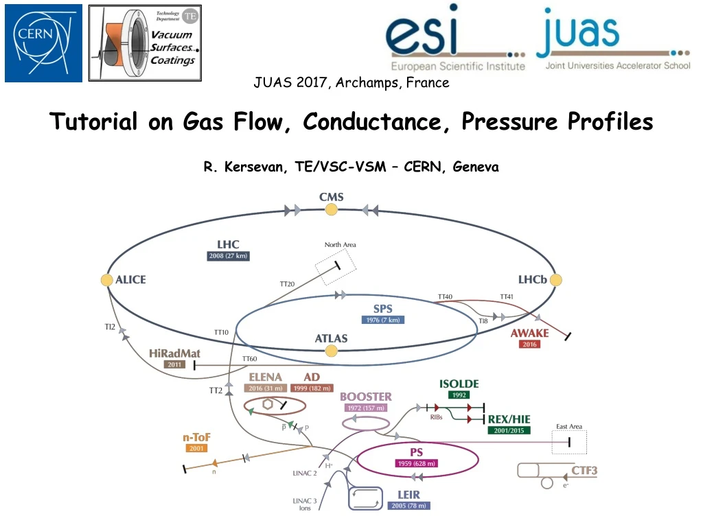
JUAS 2017, Archamps, France Tutorial on Gas Flow, Conductance, Pressure Profiles R. Kersevan, TE/VSC-VSM – CERN, Geneva
Content: • Concepts of gas flow, conductance, pressure profile as relevant to the design of the vacuum system of modern accelerators; • A quick definition of the terms involved; • Some computational models and algorithms: analytical vs numerical; • Simple exercises (if times allows) • Summary;
Sources: “[1] Fundamentals of Vacuum Technology”, Oerlikon-Leybold (*); [2] “Vacuum Technology, A. Roth, Elsevier; [3] “A User’s Guide to Vacuum Technology”, J.F. O’Hanlon, Wiley-Interscience; [4] “Vacuum Engineering Calculations, Formulas, and Solved Exercises”, A. Berman, Academic Press; Tutorial on Gas Flow, Conductance, Pressure Profiles • (*) Not endorsing products of any kind or brand 2
Sources: [5] “Handbook of Vacuum Technology”, K. Jousten ed., Wiley-Vch, 1002 p. Tutorial on Gas Flow, Conductance, Pressure Profiles 3
Units and Definitions Tutorial on Gas Flow, Conductance, Pressure Profiles 4
Units and Definitions [2] • Without bothering Democritus, Aristoteles, Pascal, Torricelli et al… a modern definition of “vacuum” is the following (American Vacuum Society, 1958): • “… given space or volume filled with gas at pressures belowatmospheric pressure” • Keeping this in mind, the following curve [2] defines the molecular densityvspressure and the mean free path (MFP), a very important quantity: • Mean-free path: average distance • travelled by a molecule before hitting • another one (ternary, and higher-order, collisions are negligible) • The importance of obtaining a low pressure, in accelerators, is evident: • - reduce collisions between the particle beams and the residual gas; • - increase beam lifetime; • - reduce losses; • - reduce activation of components; • - reduce doses to personnel; • - decrease number of injection cycles; • - improve beam up-time statistics; • - more.. Tutorial on Gas Flow, Conductance, Pressure Profiles 5
Units and Definitions [3] • A different view can be found here… • http://hyperphysics.phy-astr.gsu.edu/hbase/kinetic/menfre.html Tutorial on Gas Flow, Conductance, Pressure Profiles More molecular dimensions, dm, can be found here: http://www.kayelaby.npl.co.uk/general_physics/2_2/2_2_4.html 6
Units and Definitions [4] Definition of “flow regime” The so-called “Knudsen number” is defined as this: And the different flow (pressure) regimes are identified as follows: FREE MOLECULAR FLOW : Kn >1 TRANSITIONAL FLOW : 0.01< Kn< 1 CONTINUUM (VISCOUS) FLOW: Kn< 0.01 Practically all accelerators work in the free-molecular regime i.e. in a condition where the MFP l is bigger than the “typical” dimension of the vacuum chamber (e.g.its diameter), and therefore molecular collisions can be neglected. Tutorial on Gas Flow, Conductance, Pressure Profiles IMPORTANT: in molecular flow regime, the absence of collisions between molecules translates into the fact that high-vacuum pumps DO NOT “SUCK” GASES, they simply generate some probability s that once a molecule enters into the pump it is permanently removed from the system. s can be identified as the equivalent sticking coefficient. 7
Units and Definitions [5] Definition of “vacuum ranges” • Linked to the Knudsen number and the flow regimes, historically defined as in table below [1]; • With the advent of very low-outgassing materials and treatments (e.g. NEG-coating), “Ultrahigh vacuum” (UHV) is sometimes split up in “UHV” and “XHV” (eXtreme High Vacuum) regimes • (Ref. N. Marquardt, CERN CAS 1999) Tutorial on Gas Flow, Conductance, Pressure Profiles 8
Impingement and Collision rates; Ideal Gas Law • Impingement rate and collision rates • The ideal gas law states that the pressure P of a diluted gas is given by … where: V = volume, m3; m = mass of gas, kg M = molecular mass, kg/mole T = absolute temperature, °K R = gas constant = 8.31451 J/mol/K nM = number of moles NA = Avogadro’s number = 6.022E+23 molecules/mole kB = Boltzmann’s constant = 1.381E-23 J/K • Deviation from this law are taken care of by introducing higher-order terms, the so called virial expansion,… … which are not discussed here. Tutorial on Gas Flow, Conductance, Pressure Profiles 9
Volumetric Flow Rate – Throughput – Basic Equations - Conductance • How does all this translates into “accelerator vacuum”? • Let’s imagine the simplest vacuum sistem, a straight tube with constant cross-section connecting two large volumes, P1>P2 • Q= P·dV/dt • Q, which in the SI has the units of • [Pa·m3/s] [N·m /s] = [J/s] = [W] • … is called the throughput. Therefore the throughput is the power carried by a gas flowing out (or in) of the volume V at a rate of dV/dt and pressure P. • dV/dt is also called “volumetric flow rate”, and when applied to the inlet of a pump, it is called “pumping speed”. • Therefore, we can also write a first basic equation of vacuum technology • Q= P·S • Having defined the throughput, we move now to the concept of conductance, C: Suppose we have two volumes V1 and V2, at pressures P1>P2 respectively, connected via a tube …we can define a second basic equation of vacuum technology Q= C·(P1-P2)= C·DP … which, making an electrical analogy… I= V / R … gives an obvious interpretation of C as the reciprocal of a resistance to flow. The higher the conductance the more “current” (throughput) runs through the system. Q P1 P2 Tutorial on Gas Flow, Conductance, Pressure Profiles 10
Kinetic Theory of Gases • How can conductances be calculated? How does the dimension, shape, length, etc… of a vacuum component define its conductance? • We need to recall some concepts of kinetic theory of gases: • The Maxwell-Boltzmann velocity distribution defines an ensemble of N molecules of given mass m and temperature T as • … with n the molecular density, and kb as before. • The shape of this distribution for air at different temperatures, and for different gases at 25°C are shown on the right: Tutorial on Gas Flow, Conductance, Pressure Profiles 11
Kinetic Theory of Gases [2] • The kinetic theory of gases determines the mean, most probable, and rms velocity as: … with R the gas constant (J/°K/mole), M the molecular weight (kg/m3), and T the absolute temperature (°K). Therefore, vmp< vmean< vrms. For air at 25°C these values are: mp = 413 m/s vmean= 467 m/s vrms = 506 m/s For a gas with different M and T, these values scale as The energy distribution of the gas is Tutorial on Gas Flow, Conductance, Pressure Profiles 12
Transmission probability • Within the kinetic theory of gases, it can be shown that the volumetric flow rate passing through an infinitely thin hole of surface area A between two volumes is given by ... and by the analogy with the second basic equation we get that the conductance c of this thin hole is For holes which are not of zero-thickness, a “reduction” factor k, 0<k<1, can be defined. K is called transmission probability, and can be visualized as the effect of the “side wall” generated by the thickness. It depends in a complicated way from the shape of the hole. So, in general, for a hole of area A across a wall of thickness L Zero-thickness vs finite-thickness aperture in a wall… … the transmission probability decreases as L increases… Tutorial on Gas Flow, Conductance, Pressure Profiles L 13
Transmission probability [2] • Only for few simple cross-sections of the hole, an analytic expression of k(A,L) exists. • For arbitrary shapes, numerical integration of an integro-differential equation must be carried out, and no analytical solution exists: (ref. W. Steckelmacher, Vacuum 16 (1966) p561-584) Tutorial on Gas Flow, Conductance, Pressure Profiles 14
Sum of Conductances • Keeping in mind the interpretation of the conductance as the reciprocal of a resistance in an electric circuit, we may be tempted to use “summation rules” similar to those used for series and parallel connection of two resistors. • It turns out that these rules are not so far off, they give meaningful results provided some “correction factors” are introduced • parallel • series • and they can be extended to more elements by adding them up. • The correction factor takes into account also the fact that the flow of the gas as it enters the tube “develops” a varying angular distribution as it moves along it, even for a constant section. • At the entrance, the gas crosses the aperture with a “cosine distribution”_ …while at the exit it has a so called “beamed” distribution, determined by the collisions of the molecules with the side walls of the tube, as shown above (solid black line) • As the length of the tube increases… q F(q)≈cos(q) Tutorial on Gas Flow, Conductance, Pressure Profiles 15
Molecular Beaming Effect … at the entrance of the tube, and then follows their traces until they reach the exit of the tube. • Time is not a factor, and residence time on the walls is therefore not an issue. • Each collision with the walls is followed by a random emission following, again, the cosine distribution… • … this is repeated a very large number of times, in order to reduce the statistical scattering and apply the large number theorem. • The same method can be applied not only to tubes but also to three-dimensional, arbitrarily-shaped compo-nents, i.e. “models” of any vacuum system. • In this case, pumps are simulated by assigning “sticking coefficients” to the surfaces representing their inlet flange. • The sticking coefficient is nothing else than the probability that a molecule… … so does the beaming, and the forward- and backward-emitted molecules become more and more skewed, as shown here… • The transmission probability of any shape can be calculated with arbitrary precision by using the Test-Particle Montecarlo method (TPMC). • The TPMC generates “random” molecules according to the cosine distribution… Tutorial on Gas Flow, Conductance, Pressure Profiles 16
Effective Pumping Speed … hitting that surface gets pumped, i.e. removed from the system. • The equivalent sticking coefficients of a pump of pumping speed S [l/s] represented by an opening of A [cm2] is given by … i.e. it is the ratio between the given pumping speed and the conductance of the zero-thickness hole having the same surface area of the opening A. • The “interchangeability” of the concept of conductance and pumping speed, both customarily defined by the units of [l/s] (or [m3/s], or [m3/h]), suggests that if a pump of nominal speed Snom [l/s] is connected to a volume V via a tube of conductance C, the effective pumping speed of the pump will be given by the relationship • From this simple equation it is clear that it doesn’t pay to increase the installed pumping speed much more than the conductance C, which therefore sets a limit to the achievable effective pumping speed. • This has severe implications for accelerators, as they typically have vacuum chambers with a tubular shape: they are “conductance-limited systems”, and as such need a specific strategy to deal with them Tutorial on Gas Flow, Conductance, Pressure Profiles 17
Transmission Probability and Analytical Formulae • The transmission probability of tubes has been calculated many times. This paper (J.Vac.Sci.Technol. 3(3) 1965 p92-95)… … gives us a way to calculate the conductance of a cylindrical tube of any length to radius ratio L/R >0.001: … where Ptransm is the transmission probability of the tube, as read on the graph and 11.77 is the “usual” kinetic factor of a mass 28 gas at 20°C. • Other authors have given approximate equations for the calculation of Ctransm, namely Dushman (1922), prior to the advent of modern computers … with D and L in m. • We can derive this equation by considering a tube as two conductances in series: CA, the aperture of the tube followed by the tube itself, CB. • By using the summation rule for…. Tutorial on Gas Flow, Conductance, Pressure Profiles 18
Dushman’s Formula for Tubes … 2 conductances in series… … we obtain: and … with D and L in cm. Substituting above… Beware: the error can be large! • Exercise: 1) estimate the conductance of a tube of D=10 [cm] and L=50 [cm] by using the transmission probability concept and compare it to the one obtained using Dushman’s formula. 2) Repeat for a tube with L=500 [cm]. 3) Calculate the relative error. • This fundamental conductance limitation has profound effects on the design of the pumping system: the location, number and size of the pumps must be decided on the merit of minimizing the average pressure seen by the beam(s). • The process is carried out in several steps: first a “back of the envelope” calculation with evenly spaced pumps, followed by a number of iterations where the position of the pumps and eventually their individual size (speed) are customized. • Step one resembles to this: a cross-section common to all magnetic elements is chosen, i.e. one which fits inside all magnets (dipoles, quadrupoles, sextupoles, etc…): this determines a specific conductance for the vacuum chamber cspec (l·m/s), by means of, for instance, the transmission probability method. Tutorial on Gas Flow, Conductance, Pressure Profiles 19
{ { Pressure Profiles and Conductance • We then consider a chamber of uniform cross-section, of specific surface A [cm2/m], specific outgassing rate of q [mbar·l/s/cm2], with equal pumps (pumping speed S [l/s] each) evenly spaced at a distance L. The following equations can be written: …which can be combined into … with boundary conditions … to obtain the final result L Tutorial on Gas Flow, Conductance, Pressure Profiles 20
Pressure Profiles and Conductance [2] • From this equation for the pressure profile, we derive three interesting quantities: the average pressure, the peak pressure, and the effective pumping speed as: • From the 1st and 3rd ones we see that once the specific conductance is chosen (determined by the size of the magnets, and the optics of the machine), how low the average pressure seen by the beam can be is limited by the effective pumping speed, which in turn depends strongly on c. • The following graph shows an example of this: for c=20 [l·m/s] and different nominal pumping speeds for the pumps, the graphs show how Seff would change. • This, in turn, determines the average… pump spacing, and ultimately the number of pumps. • Summarizing: in one simple step, with a simple model, one can get an estimate of the size of the vacuum chamber, the number and type of pumps, and from this, roughly, a first estimate of the capital costs for the vacuum system of the machine. Not bad! Tutorial on Gas Flow, Conductance, Pressure Profiles 21
Pressure Profiles and Conductance [3] • So, the conductance limitation leads to the need to install many smaller pumps rather than a few large ones, as highlighted here below: (analytical calculation as per ) O. Seify, Iranian Light Source, personal comm. Tutorial on Gas Flow, Conductance, Pressure Profiles 22
Pressure Profiles and Conductance [3] • Same as previous one, but calculated via TPMC simulation, Molflow+: Q=1 mbar·l/s for each of the 3 tubes; L=8 m; Sinst=300 l/s; 1, 2, and 4 pumps; P = Q/Seff Q=1 Seff=1/P Tutorial on Gas Flow, Conductance, Pressure Profiles 23
Pressure Profiles and Distributed Pumping • From the previous analysis it is clear that there may be cases when either because of the size of the machine or the dimensions of (some of its) vacuum chambers, the number of pumps which would be necessary in order to obtain a sufficiently low pressure could be too large, i.e. impose technical and cost issues. One example of this was the LEP accelerator, which was 27 km-long, and would have needed thousands of pumps, based on the analysis we’ve carried out so far. • So, what to do in this case? Change many small pumps into one more or less continuous pump, i.e. implement distributed pumping. • In this case if Sdist is the distributed pumping speed, its units are [l/s/m], the equations above become: • We obtain a flat, constant, pressure profile. • The distributed pressure profile in LEP had been obtained by inserting a NEG-strip along an ante-chamber, running parallel to the beam chamber, and connected by small oval slots: Tutorial on Gas Flow, Conductance, Pressure Profiles 24
Pressure Profiles and Distributed Pumping [2] Effect on pressure profile of Sdist: the parabolic pressure bumps are flattened • Exercise: knowing that one metre of NEG-strip and the pumping slots provide approximately 294 [l/s/m] at the beam chamber, derive the equivalent number of lumped pumps of 500 [l/s] which would have been necessary in order to get the same average pressure. (see p.20-21) • Input data: • Cspec(LEP) = 100 [l·m/s] • Sdist(LEP) = 294 [l/s/m] • ALEP = 3,200[cm2/m]; • q = 3.0E-11 [mbar*l/s/cm2] • Exercise: the SPS transfer line has a vacuum pipe of 60 [mm] diameter, and the distance L between pumps is ~ 60 [m]. The pumping speed of the ion-pumps installed on it is ~ 15 [l/s] at the pipe. Assuming a thermal outgassing rate q=3E-11 [mbar·l/s/cm2] calculate: • 1) Pmax, Pmin, Pavg, in [mbar] • 2) Seff, in [l/s] Tutorial on Gas Flow, Conductance, Pressure Profiles 25
A modern way to calculate the effective pumping speed of the 20x9 mm2 racetrack pumping slots in LEP is via the Test-Particle Montecarlo method (TPMC): SNEG= 300 [l/s/m] • A virtual “test facet” is laid across the chamber’s cross-section and the pressure profile is calculated by recording all the rays crossing it; It is then possible to calculate Seff(l/s/m) and from this Cslot [l/s/m] by using the formula shown here above. • The goal is to maximize Cslot and therefore Seff without affecting too much the beam; 50x71 mm2 ante-chamber w/ NEG strip 130x71 mm2 beam chamber Tutorial on Gas Flow, Conductance, Pressure Profiles e- 26
Vacuum chamber geometries of arbitrary complexity can also be designed and analysed via the TPMC method; • In this case a model can be made with a CAD software, exported in STL format to the TPMC code Molflow+, and then the vacuum properties can be assigned to the different facets, such as outgassing rate, sticking coefficient (equivalent pumping speed), opacity (ratio of void-to-solid, to simulate fine grids, for instance), and more…; • This example shows the recent analysis of a potential new design of an injection septum magnet for the PS accelerator at CERN (model courtesy of J. Hansen, CERN-TE-VSC); Pressure gauge • At each facet no.i of the model, the local apparent pumping speed Sapp,ican be estimated from the local pressure Pi, via the simple formula: (Q=total gas load) Pumping port Snom=240 l/s Sapp = 2100 l/s Pulsed magnet Tutorial on Gas Flow, Conductance, Pressure Profiles Injected beam PS • The TPMC method “automatically” takes into account the conductance of the different parts, with no need to pre-calculate them and then plug-in their value in a finite-element or analytic formula; Ion-pumps 27
Summary: • During this short tutorial we have reviewed some important concepts and equations related to the field of vacuum for particle accelerators. • We have seen that one limiting factor of accelerators is the fact that they always have long tubular chambers, which are inherently conductance limited. • We have also seen some basic equations of vacuum, namely the P=Q/S which allows a very first glimpse at the level of pumping speed S which will be necessary to implement on the accelerator in order to get rid of the outgassing Q, with the latter depending qualitatively and quantitatively on the type of accelerator (see V. Baglin’s lessons on outgassing and synchrotron radiation, this school). • Links between the thermodynamic properties of gases and the technical specification of pumps (their pumping speed) as been given: the link is via the equivalent sticking coefficient which can be attributed to the inlet of the pump. • One simple model of accelerator vacuum system, having uniform desorption, evenly spaced pumps of equal speed has allowed us to derive some preliminary but useful equations relating the pressure to the conductance to the effective pumping speed, and ultimately giving us a ballpark estimate about the number of pumps which will be needed in our accelerator. • An example of a real, now dismantled, accelerator has been discussed (LEP), and the advantages of distributed pumping vs lumped pumping detailed. • Two examples of a more modern way of calculating conductances and pressure profiles (TPMC) have been shown: it should be the preferred method for the serious vacuum scientist; Tutorial on Gas Flow, Conductance, Pressure Profiles 28
References (other than those given on the slides): • P.Chiggiato, proceedings JUAS 2012-2016 • V. Baglin, proceedings JUAS 2017 • M. Ady, PhD thesis EPFL, https://cds.cern.ch/record/2157666?ln=en • R. Kersevan, M. Ady: http://test-molflow.web.cern.ch/ • CAS – CERN Accelerator School: Vacuum Technology, Snekersten (DK), 1999, https://cds.cern.ch/record/402784?ln=fr • R. Kersevan, “Vacuum in Accelerators”, Proc. CAS Vacuum, Platja d’Aro, 2006, https://cas.web.cern.ch/cas/Spain-2006/Spain-lectures.htm • M. Ady et al., “Propagation of Radioactive Contaminants Along the Isolde Beamline”, Proc. IPAC 2015, Richmond, USA, 2015 https://cds.cern.ch/record/2141875/files/wepha009.pdf • Y. Li et al.: “Vacuum Science and Technology for Accelerator Vacuum Systems”, U.S. Particle Accelerator School, Course Materials – Old Dominion University - January 2015; http://uspas.fnal.gov/materials/15ODU/ODU-Vacuum.shtml Thank you for your attention Tutorial on Gas Flow, Conductance, Pressure Profiles