Download

1 / 17
170 likes | 326 Views
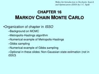
Slides for Introduction to Stochastic Search and Optimization ( ISSO ) by J. C. Spall. CHAPTER 16 M ARKOV C HAIN M ONTE C ARLO. Organization of chapter in ISSO Background on MCMC Metropolis-Hastings algorithm Numerical example of Metropolis-Hastings Gibbs sampling

E N D
Slides for Introduction to Stochastic Search and Optimization (ISSO)by J. C. Spall CHAPTER 16MARKOV CHAINMONTECARLO Organization of chapter in ISSO Background on MCMC Metropolis-Hastings algorithm Numerical example of Metropolis-Hastings Gibbs sampling Numerical example of Gibbs sampling Optional in these slides: Non-Gaussian state estimation (not in ISSO)
Background • Process generating random vector X, • Want to compute E([f(X)] for function f() • Standard method for approximating E([f(X)] is to generate many independent sample values of X and compute sample mean of f(X) values • Only useful in “trivial” cases where X can be generated directly • Many practical problems have non-trivial distribution for X • E.g., state in nonlinear/non-Gaussian state-space model
Markov Chains • Not necessary to generate independent X to estimate E([f(X)] • Consider dependentsequence X0, X1, X2,… • Generate Xk+1 according to “easy” conditional distribution for {Xk+1|Xk} • {Xk} process is a Markov chain • Xk dependence on fixed number of early states disappears as k gets large • Above implies distribution of Xk approaches a stationary form as k gets large • Stationary form corresponds to target distribution (density) p(·) if conditional distribution chosen properly
Ergodic Averaging • Let M denote the “burn-in” period for the Markov chain • The ergodic average of n – M values of f(X) with Xkgenerated via a Markov chain is • Summands above are dependent via the Markov property for the {Xk} • Above sum approaches E([f(X)] as n gets large by ergodic theorem
Metropolis-Hastings (M-H) Algorithm • M-H algorithm is one of two most popular forms for MCMC (other is Gibbs sampling) • M-H relies on proposal distribution and Metropolis criterion • Let proposal distribution be q(·|·); used to generate candidate pointsW ~q(·|X=x) • Candidate point W = w is accepted with probability given by Metropolis criterion: • In practice, in going from Xk toXk+1, x above is Xk and W becomes Xk+1 if W is accepted
M-H Algorithm for Estimating E([f(X)]) Step 0 (initialization)Choose length of “burn-in” period M and initial state X0. Set k = 0. Step 1 (candidate point) Generate a candidate point W according to proposal distribution q(|Xk). Step 2 (accept/reject) Generate point U from U(0,1) distribution. Set Xk+1 = W if U(Xk,W) (Metropolis criterion). Otherwise set Xk+1 = Xk. Step 3 (iterate) Repeat Steps 1 and 2 until XM is available. Terminate “burn-in” process and proceed to step 4 with Xk = XM. Steps 4–6 (ergodic average)Repeat process and compute average of f(XM+1),…, f(Xn). This ergodic average is estimate of E([f(X)].
Example: Estimating E([f(X)]) from a Bivariate Normal Distribution(Example 16.1 from ISSO) • Suppose • Use M-H to estimate sum of the two mean components (true value = 0):f(X) = [1,1]X • Standard (unit length) uniform proposal distribution and burn-in period of M = 500 • Following plot shows three independent runs • Acceptance rate (Metropolis criterion) about 70% • Better performance possible with lower acceptance rate (requires “tuning”—not always feasible in practice)
Example (cont’d): M-H Algorithm with Uniform Proposal Distribution; Mean Zero Target 3 2 1 0 –1 –2 –3 0 5000 10000 15000 Iterations (Post Burn-In)
Gibbs Sampling • Gibbs sampling is implementation of M-H on element-by-element basis • Gibbs sampling uniquely designed for multivariate problems, i.e., dim(X) 2 • Gibbs sampling based on idea of “full conditional” distributions • ith full conditional distribution is conditional distribution for ith component of X conditioned on most recent values of all other components of X • In contrast to M-H, Gibbs sampling updates components of X one-at-a-time
Relationship of Gibbs Sampling to M-H • Gibbs sampling is special case of M-H on element-by-element basis • Gibbs sampling and M-H developed largely independent of each other • M-H introduced in Hastings (1970) as implementation of Metropolis sampling from statistical physics • Gibbs introduced in Tanner and Wong (1987) and Gelfand and Smith (1990), with special focus on Bayesian problems • Gibbs sampling uses particular form of full conditionals as proposal distribution from M-H • Eliminates need to “tune” proposal distribution as in general M-H • Requires stronger assumptions to construct full conditionals • Acceptance rate for new points is 100%
Example: Truncated Exponential Distribution (Example 16.5 from ISSO) • Consider two-variable problem where conditional random variables {X|Y} and {Y|X} have exponential distributions over finite interval (length = 5) • Distributions for {X|Y} and {Y|X} are two full conditionals for Gibbs sampling • Suppose interested in marginal distribution for X • Can determine exact marginal distribution for X • Useful for comparison purposes; not usually available in practice • Plot shows Gibbs output relative to true density for X • Histogram based on terminal X value from 5000 independent replications • Burn-in period of M = 10; terminal value occurs 30 iterations past burn-in
Example (cont’d): Histogram of Gibbs Sampling Output vs. Known Density
Optional (not in ISSO): Non-Gaussian State Estimation • Consider state-space model with non-Gaussian noises (xk is state; zk is measurement) • Represent p(xk|xk–1) and p(zk|xk) as Gaussian mixtures • Gaussian mixtures can be used to approx. many non-Gaussian distributions • Gibbs sampling used to estimate state based on Gaussian full conditionals • Further information on pp. 4344 of: Spall, J. C. (2003), “Estimation via Markov Chain Monte Carlo,” IEEE Control Systems Magazine, vol. 23(2), pp. 3445
Non-Gaussian State Estimation: Basic Idea • Let represent parameters in Gaussian mixture • Xn and Zn are complete collection of all (n) states and measurements • Gibbs sampling operates from full conditionals: {xk| xk–1, , Zn}— Gaussian distribution { | Xn, Zn}— non-Gaussian distribution • Above non-Gaussian distribution known for many cases • Iterative sampling from above full conditionals produces samples fromp(xk|Zn) for all k Average the samples to getE(xk|Zn)
Concluding Remarks • M-H and Gibbs sampling two notable examples of MCMC • Methods for “easy” generation of random samples and estimates • M-H more general, but Gibbs especially useful in specific applications • Not “magic”—still need relevant assumptions • Widespread use in statistics, computer science, simulation, etc. • Limited current use in control and signal processing • But non-Gaussian/nonlinear state estimation one growing area
Exercise 16.3: Four replications of M-H Algorithm with Mean Zero Target
Exercise 16.8: Histogram (2000 samples) and Known Density for X