Finite Element Method Programming: Applications and Considerations
780 likes | 801 Views
Explore the practical applications and programming considerations of one-dimensional problems using Fortran and Maple. Learn about governing equations, finite element implementation, and analysis techniques including static, time-dependent, eigenvalue, and buckling analysis. This comprehensive guide covers structural and temporal problem types, shape functions, boundary conditions, matrix solvers, and programming variables. Discover how to utilize libraries in Maple for efficient programming and gain insights into designing and analyzing various engineering systems.

Finite Element Method Programming: Applications and Considerations
E N D
Presentation Transcript
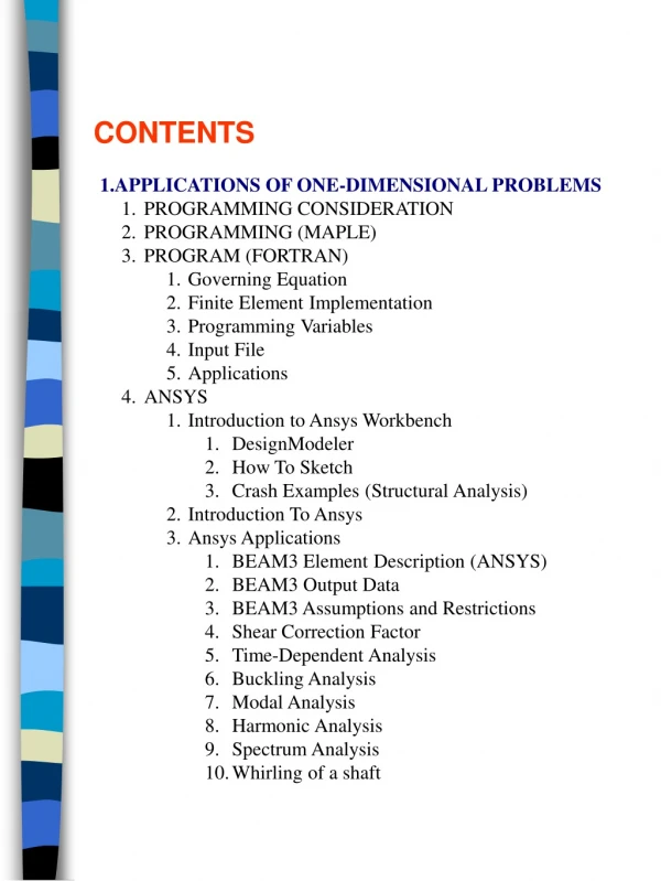
CONTENTS • APPLICATIONS OF ONE-DIMENSIONAL PROBLEMS • PROGRAMMING CONSIDERATION • PROGRAMMING (MAPLE) • PROGRAM (FORTRAN) • Governing Equation • Finite Element Implementation • Programming Variables • Input File • Applications • ANSYS • Introduction to Ansys Workbench • DesignModeler • How To Sketch • Crash Examples (Structural Analysis) • Introduction To Ansys • Ansys Applications • BEAM3 Element Description (ANSYS) • BEAM3 Output Data • BEAM3 Assumptions and Restrictions • Shear Correction Factor • Time-Dependent Analysis • Buckling Analysis • Modal Analysis • Harmonic Analysis • Spectrum Analysis • Whirling of a shaft
PROGRAMMING CONSIDERATION Model Equation Natural Coordinates • Approximate Solution and Shape Functions • Two-Node (Linear) Element
Three-Node (Quadratic) Element • Four-Node (Cubic) Element
1. Static Problems 2. Time-Dependent Problems 3. Eigenvalue Problems STRUCTURE of 1D FEM PROGRAM Observe carefully HOW the elemental stiffness matrix and force vector are computed and stored in arrays in STIFF subroutine
Applications with Maple Programs To demonstrate the programming for FEM, a complete set of functions called procedures in Maple is presented along with a main program in Appendix D. Maple has two different types; Classic Worksheet Maple and Standard Maple. There exist some differences between them. One major difference is that the former stores all executed variables and procedures into the memory that are available to any open files while the latter stores them in each file memory (not available to other files). The procedures (i.e., functions or subroutines) can be run once to put them in the memory to use. Alternatively, they can be stored in a library and called anytime to use. The provided programs are stored in three separate files; function file, application file (main program), and input file.
Creating a Library > #define a new libname (mee480.lib) to save procedures savelibname:="c:/my/maplelib/mee480.lib"; #first time, create the library march('create',savelibname); Error, (in march) there is already an archive in "c:/my/maplelib/mee480.lib" > #you can list the names of procedures if you wish listrep := r -> map2( op, 1, march( 'list', r ) ): listrep(savelibname);
Saving procedures into a Library > #copy a matrix into another one AtoB:=proc(A) Matrix(A); end proc: #copy a vector into another one XtoY:=proc(X) Vector(X); end proc: savelib('AtoB','XtoY'):
Calling a Library > #call library names to use libname:={libname,"c:/my/maplelib/mee480.lib"}[];
Governing Equation Finite Element Implementation • Temporal Types of Problems • steady state problems • first-order time dependent problems • second-order time dependent problems • first-order eigenvalue problems • second-order eigenvalue problems • Spatial Types of Problems • second order problems • fourth order problems • 2D structural problems • Shape Functions • linear shape function • quadratic shape function • cubic shape function • Boundary Conditions • essential boundary conditions • natural boundary conditions • mixed boundary conditions • constraint boundary conditions • Matrix Solver • full matrix solver • compressed matrix solver • symmetric banded matrix solver • nonsymmetric banded matrix solver • general eigenvalue solver
Programming Variables ielem indicator for the type of finite element: 2-node element for second-order problems 3-node element for second-order problems 4-node element for second-order problems 2-node element for fourth-order problems 2-node element for beam structural problems 2-node element for truss structural problems item item=0, static (not time-dependent) analysis first-order time derivatives second-order time derivatives involved eigenvalue problem for first-order in time eigenvalue problem for second-order in time buckling problems [10/26/94] must be used only with ielem=4 for=3,4,5, it outputs [K] & [M] for eigen solver icont.....indicator for continuity of the data (0, no;1, yes) icood .. flag for generation of coordinates +/- localx .. flag for local x-coordinates to use when localx > 0 or global when localx = 0 in expression of a(x),b(x),c(x) and f(x) in the differential equation nprint .. indicator for print (nprnt=n) or noprnt (nprnt=0) of the element matrices and global matrices ifmt .... indicator for print format. 0 for scientific format and 1 for floating-point format aL........length of the domain x0 ...... starting coordinate for domain ax0,ax1,ax2 bx0,bx1,bx2....coefficients in the differential equation(see stiff) cx0,cx1,cx2 (depending on LOCAlX, they are evaluated in local or global) fx0,fx1,fx2 when ielem=5, f(x) is for beam transverse load, NOT for axially distributed load Tcoeff,Tchange used with ielem=1,5,6 only coef(i,j).array for storing ax0,ax1,ax2, ...,fx0,fx1,fx2,Tcoeff(=),Tchange(=T), ax0=coef(i,1),ax1=coef(i,2), etc. for i-the element. This is used when icont = 0 (not continuous data)
Programming Variables (contd) dt........time increment for time-dependent problems maxtim.....number of time steps (in the transient analysis) alpha,beta, a1,a2,a3,a4..parameters in the time approximation schemes glx() ... array of global coordinates, x[,y] elx.......element coordinates to transfer to 'stif' gstif.....global (that is, assembled) coefficient matrix in banded form (neq x hbw) gmass ... glocal mass matrix for time-dependent and eigenvalue problems gf........columm vector of the global forces before going to the subroutine 'solve', and contains the solution when comes out of the subroutine 'solve' gf0 .... colum vectors for initial conditions on ui and its gf1,gf2 derivatives (gf1=d(u)/dt,gf2=dd(u)/dtt) elf.......element force vector nebc......number of specified primary degrees of freedom iebc......colum of specified primary degrees of freedom vebc......colum of specified values of the entris in iebc nnbc.......number of specified secondary degrees of freedom OR flag: when eigenproblem, if this is positive, the eigenvalues are sorted in ascending order. inbc.......colum of specified secondary degrees of freedom Vnbc…..collum of specified values of the entries in inbc nconv ....number of convection type problem iconv() ..node numbers for nconv vconv(,2) values of conv bcs with hconv and tinf nconst ...number of constraint conditions ipconst() vector to store the number of positions in each group iconst() vector to store the position numbers for constrain conditions vconst()..vector to store the coefficients of constraint relations
Programming Variables (cont’d) nstress...number of points in each element to compute derivatives which are related to internal loadings (must be nstress <= neq) nplot .. number of nodes to get plotting data in time-dependent problem For steady-state second-order problems, it will write position and primary variables into the plot file. iplot(i)..equation numbers where to get plotting data for transient case for steady state case, not used • nrow .... row-dimension of 'gstif' in dimension statement • ncol .... colum-dimension'gstif' in dimension statement • npe.......number of nodes per element • ndf.......number of degrees of freedom per node • nem.......number of elements in the mesh • nnm.......number of nodes in finite element mesh • neq..... total degrees of freedom in the finite element model • nhbw......half band width ofthe global coefficient matrix • ngp.......number of gauss points used in theintegration • nn........number of total degrees of freedom in the element • irel .... scale factor of displacements to coord. to plot deformed shape only in structural shape • matsym .. flag for type of global matrix used for solution and internally used. • 0 full matrix • compressed full matrix without EBC's • full matrix • non-symmetric banded matrix • symmetric banded matrix • nod(i,j) global node number correspondingto thej-th node of the i-th element (connectivity matrix) FIlES *.out......general output file *.vec......generate eigenvectors to plot mode shapes *.eig.......eigenvalues are stored for plot ** note for eigenproblems, if nplot > 0, they are sorted. *.dat.......time dependent responses at positions specified by nplot and iplot() for plot for steady state, position and primary values for plot *.bnd…...stores displacements, and its derivatives for plot in bending *.shp……original shape of the structure for plot
INPUT FILE title for informational purpose 2 4 0 1 0 0 1 0 item,ieLem,icont,localx,icood,irel,nprint,ifmt 2 3 nem,nnm 2 nebc 1 2 (IEBC(I),I=1,NEBC) 2*0 (VEBC(I),I=1,NEBC) 1 nnbc 5 (INBC(I),I=1,NNBC) -100 (VNBC(I),I=1,NNBC) 0 nconv 3 iconv() 1 0 vconv() 0 0 nconst,ipconst() 3 iconst() 1 2 0 vconst(,ndf) 3 2 nstress ,nplot 3 4 iplot() 0.5 .125 .05 20 ,,t,maxtime 0 0.1 0.2 0.3 0.4 0.5 (gf0(i),i=1,neq) 6*0 (gf1(i),i=1,neq) 0 0 0 3e6 0 0 0 0 0 -10 0 0 0 0 1 a0,a1,a2, b0,b1,b2, c0,c1,c2, f0,f1,f2, alpha,dT, c1 (or c2) 0 0 0 3e6 0 0 0 0 0 0 0 0 0 0 1 a0,a1,a2, b0,b1,b2, c0,c1,c2, f0,f1,f2, alpha,dT, c1 (or c2) 1 1 2 NOD for element 1 2 2 3 NOD for element 2 1 0 0 x1,y1 2 6 0 x2,y2 3 10 0 x3,y3
Application Ex.6.2.1 Solve the following differential equation with two linear elements • Input Data Example 0 1 1 0 1 1 0 0 item,ieLem,icont,localx,icood,irel,nprint,ifmt 2 3 nem,nnm 1 nebc 1 (IEBC(I),I=1,NEBC) 0 (VEBC(I),I=1,NEBC) 1 nnbc 3 (INBC(I),I=1,NNBC) 1 (VNBC(I),I=1,NNBC) 0 nconv 3 iconv() 0 vconv() 0 nconst,ipconst() 0 iconst() 1 2 0 vconst(ndf) 0 0 nstress,nplot 3 4 iplot() 0.5 0.125 0.05 20 a,b,Dt,maxtime 0 0.1 0.2 0.3 0.4 0.5 (gf0(i),i=1,neq) 6*0 (gf1(i),i=1,neq) 1 0 0 0 0 0 -1 0 0 0 0 -1 0 0 0 a0,a1,a2, b0,b1,b2, c0,c1,c2, f0,f1,f2, alpha,dT, c1 (or c2) (continuing the previous line) 1 0 L and x0
Output Data Example item(0:static,1,2:march,3,4:eigen)....= 0 eLement type(1,2,3,6: 2nd, 4,5: 4th)..= 1 icont(0:discont.a(x),.., 1: cont).....= 1 icood(0: input coords. 1: auto).......= 1 localx(0:global, 1:local) ............= 0 nprint ...............................= 0 nebc ................................= 0 nnbc ................................= 1 nconv ................................= 0 nconst ...............................= 0 no of equations ......................= 3 no. of eLements in mesh...............= 2 no of nodes in the mesh................= 3 no of deg. of freedom per node.....= 1 nhbw(half band width).................= 2 matsym(0,2:full,1:comp.F,3:nons,4:sym)= 3 ax0,ax1,ax2: .10000E+01 .00000E+00 .00000E+00 bx0,bx1,bx2: .00000E+00 .00000E+00 .00000E+00 cx0,cx1,cx2: -.10000E+01 .00000E+00 .00000E+00 fx0,fx1,fx2: .00000E+00 .00000E+00 -.10000E+01 Tcoeff,Tchange, c0: .00000E+00 .00000E+00. 10000E+01 c0 : .00000E+00 • specified essential boundary conditions: • 1 • values of specified essential boundary conditions: • .00000E+00 • specified nonzero natural boundary conditions: • 3 • values of specified natural boundary conditions: • .10000E+01 • FEM mesh follow: • .00000 .50000 1.00000 • 1 2 • 2 3 • solution of primary variables: • 1 .00000E+00 • 2 .60751E+00 • 3.11392E+01 • solution of external forces: • 1 -.12552E+01 • 2 .00000E+00 • 3 .10000E+01
Application Ex.6.2.2 Solve the following differential equation with two finite elements
Application Ex.6.2.3 For no heat generation in the body f = 0, conduction coefficient k = 25 W/m2-oC, the heat flux at r = 0 Q0 = -150 W/m2, and T = 50oC at r = 200, find the temperatures at 10, 20, 40, 80, 140, and 200m. Use linear and quadratic elements
Application Ex.6.2.4 Find the displacements and the reactions of the following composite structure that is axially loaded as shown below. Given a = 20 in and P = 50 kips
Application Ex.6.2.5 First determine the critical time step from the eigenvalue analysis of the following differential equation with one finite element and the solve it with = 0 and t = 0.7 and 0.5
Application Ex.6.2.6 Solve the following cantilever beam problem with one finite element. The bending rigidity EI = 105 lbf-in2, L = 12 inch, and P = 100 lbf
Application Ex.6.2.7 Solve the following differential equation with one finite element. Use = 0.5, = 0.25, and t = 0.05
Application Ex.6.2.8 Find the eigenvalues and the associated mode shapes of the equation in Example 6.2-7 with three finite elements. Plot the mode shapes
Application Ex.6.2.9 Solve the following problem with two elements. Use a = 8 inch, L = 12 inch, k = 100 lb/ft2, EI = 106 lbf-in2 and P = 150 lb
Application Ex.6.2.10 Two connected bars are fixed at both ends. When only the first bar is subjected to a force P and the temperature change T, find the displacement at the joint of the bars and the stresses in the bars. Use a = b = c = 4 inch, P = 100 lb, T = 50oC, 1 = 0.001 in/in-oC, E1 = 106 psi, E2 = 105 psi, A1 = 1 in2, and A2 = 1/4 in2
Application Ex.6.2.11 In the Example 6.2-10 how much force P must be exerted in order not to move the point where P is applied?
Application Ex.6.1.12 A uniformly distributed load f(x) = 200 kN/m is acting on a 500 mm rigid bar at temperature 85oC which sits on three members shown below. The member 1 and 3 are made of steel rod with 40 mm diameter and have the material properties Est = 200 GPa and st = 12 x 10-6 /oC, while the member 2 is made of aluminum rod with 60 mm diameter and has Eal = 70 Gpa and al = 23 x 10-6 /oC. When no load was applied, the temperature was 25oC. Find the forces acting on the members. The length of members is h = 250 mm.
Application Ex.6.1.13 A beam-bar structure shown below is subjected to the following loadings. Find the reaction forces and moments at supports and determine the internal loadings at point G. Given are a = 3 ft, b = 2 ft, c = 5 ft, d = 3 ft, f0 = 250 lbf/ft, and P = 1500 lb. The bars have 1 inch diameters and E = 106 psi and the beam has E = 3 x 10⁶ psi and Iyy = 1/24 in4.
Application Ex.6.2.14 Determine the reaction forces at the support A and the internal loadings at point C. Given are P = 300 lbf/ft, a = 4 ft, and b = 6 ft
ANSYS Brief Introduction To Ansys
Ex.6.3.2.1 [Ceqns] Find the displacements and the reactions of the following composite structure that is axially loaded as shown below. Given a = 20 in and P = 50 kips
Ex.6.3.2-2 [MBC] Find the displacements and the reactions of the following composite structure that is axially loaded as shown below. Given a = 20 in, b = 8 in, c = 4 in, k = 1010 lb/in, and P = 100 kips
Ex.6.3.2-3 [Distributed Load] Find the displacements and the reactions of the following beam that is loaded as shown below. Given a = 4 in, b = 6 in, k = 104 lb-in, P = 1000 lbf/in, E = 106 psi, and the cross-section of h = 2 in and w = 3/2 in