Principal Components
Principal Components . Karl Pearson. Principal Components (PC). Objective : Given a data matrix of dimensions nxp (p variables and n elements) try to represent these data by using r variables (r<p) with minimum lost of information .

Principal Components
E N D
Presentation Transcript
Principal Components (PC) • Objective: Given a data matrix of dimensions nxp (p variables and n elements) try to represent these data by using r variables (r<p) with minimum lost of information
We want to find a new set of p variables, Z, which are linear combinations of the original X variable such that : • r of them contains all the information • The remaining p-r variables are noise
First interpretation of principal components Optimal Data Representation
Proyection of a point in direction a: minimize the squared distance Implies maximizing the variance (assuming zero mean variables) ri xi zi xiTxi = riT ri+ zTi zi a
Second interpretation of PC: Optimal Prediction Find a new variable zi =a’Xi which is optimal to predict The value of Xi in each element . In general, find r variables, zi =Ar Xi , which are optimal to forecast All Xi with the least squared error criterion It is easy to see that the solution is that zi =a’Xi must have maximum variance
Third interpretation of PC Find the optimal direction to represent the data. Axe of the ellipsoid which contains the data The line which minimizes the orthogonal distance provides the axes of the ellipsoid This is idea of Pearson orthogonal regression
The analysis have been done with 16 images. PC allows that Instead of sending 16 matrices of N2 pixels we send a vector 16x3 with the values of the components and a matrix 3xN2 with the values of the new variables. We save If instead of 16 images we have 100 images we save 95%