DC breakdown measurements
400 likes | 605 Views
DC breakdown measurements . Sergio Calatroni Present team: Jan Kovermann , Chiara Pasquino , Rocio Santiago Kern, Helga Timko , Mauro Taborelli , Walter Wuensch. Outline. Experimental setup Typical measurements Materials and surface preparations Time delays before breakdown

DC breakdown measurements
E N D
Presentation Transcript
DC breakdown measurements Sergio Calatroni Present team: Jan Kovermann, ChiaraPasquino, Rocio Santiago Kern, Helga Timko, Mauro Taborelli, Walter Wuensch
Outline • Experimental setup • Typical measurements • Materials and surface preparations • Time delays before breakdown • Gas released during breakdown • Evolution of and Eb • Effect of spark energy • Future Sergio Calatroni - 19.11.2010
Experimental set-up : ‘‘ the spark system ’’ vacuum chamber (UHV 10-10 mbar) HV switch HV switch m-displacement gap 10 - 50 mm (±1 mm) 20 mm typically anode (rounded tip, Ø 2 mm) power supply (up to 15 kV) V spark cathode (plane) C (28 nF typical) • Two similar systems are running in parallel • Types of measurements : Field Emission ( b) Conditioning ( breakdown field Eb) Breakdown Rate ( BDR vs E) Sergio Calatroni - 19.11.2010
gas analyzer vacuum gauges V optical fibre V photomultiplier or spectrometer current probe HV probe to scope Experimental set-up : diagnostics V Sergio Calatroni - 19.11.2010
Field emission - measurement • An I-V scan is performed at limited current, fitting the data to the classical Fowler-Nordheim formula, where [jFE] = A/m2, [E] = MV/m and [φ] = eV (usually 4.5 eV). is extracted from the slope Sergio Calatroni - 19.11.2010
Conditioning – average breakdown field Molybdenum Copper Eb Eb Deconditioning 1-5 sparks or no conditioning Conditioning phase: 40 sparks Sergio Calatroni - 19.11.2010
Surface damage (Mo) 1 5 10 20 40 100 Sergio Calatroni - 19.11.2010
Conditioning curves of pure metals Selection of new materials for RF structure fabrication was the original purpose of the experiment Sergio Calatroni - 19.11.2010
hcp fcc : face-centered cubic bcc : body-centered cubic hcp : hexagonal closest packing bcc hcp bcc bcc bcc bcc bcc fcc fcc Breakdown field of materials (after conditioning) • In addition to other properties, also importance of crystal structure? • reminder : Cu < W < Mo same ranking as in RF tests (30 GHz) Sergio Calatroni - 19.11.2010
Surface treatments of Cu • Surface treatments on Cu only affects the very first breakdowns • After a few sparks: ~ 170 MV/m, b ~ 70 for everysamples The first sparks destroy rapidly the benefit of a good surface preparation and result in deconditioning. This mightbe the intrinsincproperty of copper surface In RF, sparksare distributed over a muchlargersurface, and conditioningisseen. Mightbe due to extrinsicproperties. • More foreseen in the near future to assess the effect of etching, brazing, etc. Sergio Calatroni - 19.11.2010
Oxidized copper • Cu2O is a p-type semiconductor, witha higherworkfunctionthan Cu : 5.37 eV instead of 4.65 eV • Cu oxidizedat 125°C for 48h in oven (air): purple surface ↔ Cu2O layer~15 nm • Cu oxidizedat 200°C for 72h in oven (air): 2 1 • BDR = 1 for standard Cu @ 300 MV/m • BDR = 10-3 – 10-4 for oxidizedCu @ 300 MV/m, but last only a few sparks Sergio Calatroni - 19.11.2010
Breakdown rate experiments • A target field value is selected and applied repeatedly for 2 seconds • BDR is as usual: #BD / total attempts • Breakdown do often appear in clusters (a simple statistical approach can account for this) Sergio Calatroni - 19.11.2010
Breakdown Rate : DC & RF (30 GHz) BDR ~ Eg Same trend in DC and in RF, difficultto compare ‘slopes’ Sergio Calatroni - 19.11.2010
Time delays before breakdown delay • Voltage rising time : ~ 100 ns • Delay beforespark : variable • Sparkduration : ~ 2 ms Sergio Calatroni - 19.11.2010
Cu Ta Mo SS Eb = 170 MV/m Eb = 300 MV/m Eb = 430 MV/m Eb = 900 MV/m R = 0.07 R = 0.29 R = 0.76 R = 0.83 R = fraction of delayed breakdowns (excludingconditioningphase, whereimediated breakdowns dominate) R increases with average breakdown field Time delays with different materials (but why ?!?) Sergio Calatroni - 19.11.2010
Correlation pre-current & delays With our simple thermal model (based on Williams & Williams J. Appl. Phys. D 5 (1972) 280) which lead to the establishment of the scaling quantity “Sc” Phys.Rev.ST-AB 12 (2009) 102001 From: Kartsev et al. SovPhys-Doklady15(1970)475 Sergio Calatroni - 19.11.2010
Gas released during a breakdown 0.95 J / spark 0.8 J / spark (heat treatment: ex-situ, 815°C, 2h, UHV) • Samegasesreleased, withsimilar ratios • Outgassingprobablydominated by Electron StimulatedDesorption (ESD) • Slightdecrease due to preliminaryheattreatment • Data used for estimates of dynamic vacuum in CLIC strucures Sergio Calatroni - 19.11.2010
consecutive breakdowns ‘quiet’ period H2outgassing in Breakdown Rate mode (Cu) Outgassingpeaksat breakdowns Slightoutgassingduring ‘quiet’ periods ESD with FE e-at the anode No visible increase in outgassingjustbefore a breakdown Sergio Calatroni - 19.11.2010
b · Eb = const b↔ next Eb correlation b↔ previous Eb no correlation b · Ebis the constant parameter (cf. Alpertet al., J. Vac. Sci. Technol., 1, 35 (1964)) Local field: · Eb (Cu) • Measurements of b after each sparks (Cu electrodes) Sergio Calatroni - 19.11.2010
conditioning ? b · Eb = 10.8 GV/m (± 16%) good surface state Local field = const= 10.8 GV/m for Cu Evolution of & Eb during conditioning experiments Eb = 159 MV/m (± 32%) b = 77 (± 36%) Sergio Calatroni - 19.11.2010
Evolution of during BDR measurements (Cu) No spark Spark • General pattern : clusters of consecutive breakdowns / quiet periods (BDR = 0.11 in this case) • bslightlyincreasesduring a quiet periodif E issufficientlyhigh The surface ismodified by the presence of the field (are « tips » pulled?) Sergio Calatroni - 19.11.2010
b·E = 10.8 GV/m Evolution of during BDR measurements (Cu) No spark Spark • Breakdown as soon as b > 48 ( ↔ b · 225 MV/m > 10.8 GV/m) • Consecutivebreakdowns as long as b > bthreshold length and occurence of breakdown clusters ↔ evolution of b Sergio Calatroni - 19.11.2010
Effect of spark energy - Cu • EBRD increases with lower energy (less deconditioning is possible) • Local breakdown field remains constant Sergio Calatroni - 19.11.2010
Effect of spark energy - Mo • EBRDseems to increase with higher energy (better conditioning possible) • Local breakdown field remains constant • However, we have doubts on representative the measurement is in this case Sergio Calatroni - 19.11.2010
Energy scaling of the spot size • The diameter of the damaged area depends on the energy available • Area mostly determined by the conditioning phase • Decreases with decreasing energy; saturates below a given threshold Mo Cu Sergio Calatroni - 19.11.2010
The future • Ongoing work: • Finalise the work on the effect of spark energy on BD field, and understand the beta measurements for Mo • Trying to understand “worms”( “flowers”?) Sergio Calatroni - 19.11.2010
The future • Effect of temperature on evolution and other properties • To verify the hypothesis and the dynamic of dislocation • Fast electronics • Defined pulse shape and duration, without and during breakdowns • Repetition rate up to 1 kHz (107 pulses -> less than 3 hours) Sergio Calatroni - 19.11.2010
Fast electronics Mike Barnes Rudi Henrique Cavaleiro Soares Sergio Calatroni - 19.11.2010
The future • Effect of surface treatment and in general of the fabrication process on BD • To study the influence of etching and its link with machining (preferential etching at dislocations, field enhancement or suppression, smoothening etc.) • To study the influence of H2 bonding (faceting, etc) • (In parallel, ESD studies on the same samples) Depends on capability of accurately measure the gap without prior surface contact Sergio Calatroni - 19.11.2010
Reoxidation 1st oxidation 150 sparks 2nd oxidation 180 sparks O element% = 3.8 • A sparked (damaged) surface was reoxidised by heating and was sparked then again • Was not able to recover the initial high EBRD • Oxidised, smooth surface high EBRD • Oxidised, sparked surface no improvement • Connection to the oxidation process? O element% = 1.0 O element% = 3.5-3.7 1st oxidation 30 sparks 2nd oxidation O element% = 1.6 O element% = 0.9-2.1 O element%=1.3-1.7 O element% = 0.3 Sergio Calatroni - 19.11.2010
Field profile on the cathode surface E • Tip – plane geometry • dependence with the gap distance x Sergio Calatroni - 19.11.2010
b · Ebis the constant parameter (cf. Alpertet al., J. Vac. Sci. Technol., 1, 35 (1964)) Gap dependence of Eb, b and b · Eb (Cu) Sergio Calatroni - 19.11.2010
Surface damage (Cu) Sergio Calatroni - 19.11.2010
Gap measurement damage Sergio Calatroni - 19.11.2010
Heating of tips by field emission - I r=radius • The tip has a height/radius (field enhancement factor) • For a given value of applied E the Fowler-Nordheim law gives a current density J(E)=A*(E)2*exp(-B/E) • This current produces a power dissipation by Joule effect in each element dz of the tip, equal to dP = (J r2)2 (z) dz / r2 • The total dissipated power results in a temperature increase of the tip (the base is assumed fixed at 300 K). The resistivity itself if temperature dependent • Using the equations we can, for example, find out for a given what is the field that brings the “tip of the tip” up to the melting point, and in what time. • Used for “Sc” derivation Phys.Rev.ST-AB 12 (2009) 102001 T = Tmelting J(E) h=height dz T = 300K Sergio Calatroni - 19.11.2010 CLIC Breakdown Workshop Sergio Calatroni TS/MME 36
Heating of tips by field emission - II • If the resistivity is considered temperature-independent, a stable temperature is always achieved [Chatterton Proc. Roy. Soc. 88 (1966) 231] • If the resistivity (other material parameters play a lesser role) is temperature dependent, then its increase produces a larger power dissipation, resulting in a further temperature increase and so on [Williams & Williams J. Appl. Phys. D 5 (1972) 280] • Below a certain current threshold, a stable regime is reached • Above the threshold, a runaway regime is demonstrated • The time dependence of the temperature can be calculated. Sergio Calatroni - 19.11.2010 CLIC Breakdown Workshop Sergio Calatroni TS/MME 37
Simulation for Mo cone: diameter 20 nm, beta = 30 E=374 MV/m E=378 MV/m High Gradient Workshop 2008
Time constant to reach the copper melting point (cylinders, =30) The tips which are of interest for us are extremely tiny, <100 nm (i.e. almost invisible even with an electron microscope) Sergio Calatroni - 19.11.2010 CLIC Breakdown Workshop Sergio Calatroni TS/MME 39
Power density at the copper melting point (cylinders, =30) Power density (power flow) during the pulse is a key issue. See talk by A. Grudiev for RF structures scaling based on Poyinting vector Sergio Calatroni - 19.11.2010 CLIC Breakdown Workshop Sergio Calatroni TS/MME 40