Comp. Genomics
Comp. Genomics. Recitation 5 2/4/09 ML in Phylogeny. Based on Slides by Ron Shamir and Nir Friedman. Outline. Maximum likelihood (ML) ML in phylogeny Ancestral sequence reconstruction using ML. Maximum likelihood. One of the methods for parameter estimation

Comp. Genomics
E N D
Presentation Transcript
Comp. Genomics Recitation 5 2/4/09 ML in Phylogeny Based on Slides by Ron Shamir and Nir Friedman
Outline • Maximum likelihood (ML) • ML in phylogeny • Ancestral sequence reconstruction using ML
Maximum likelihood • One of the methods for parameter estimation • Likelihood: L=P(Data|Parameters) • Simple example: • Simple coin with P(head)=p • 10 coin tosses • 6 heads, 4 tails • L=P(Data|Params)=(106)p6 (1-p)4
Maximum likelihood • We want to find p that maximizes L=(106)p6 (1-p)4 • Infi 1, Remember? • Log is a monotolical function, we can optimize logL=log[(106)p6 (1-p)4]= log(106)+6logp+4log(1-p)] • Deriving by p we get: 6/p-4/(1-p)=0 • Estimate for p:0.6 (Makes sense?)
Likelihood of a Tree • Input (small problem): • n sequences • A tree T, with labels on the leafs (X) • Find optimal labeled tree: • labeling of internal nodes (Y) • branch lengths (b) • Maximizing the likelihood P(X|T,Y,b)
Likelihood (2) • How to compute P(X|T,Y,b)? • Assumptions: • Each character is independent • The branching is a Markov process: • The probability of a node having a given label is only a function of the parent node and the branch length b between them. • The probabilities P(x|y,t)are known
x5 t5 x4 t3 t2 t1 x2 x1 x3 Example
What if we want P(X|T,b)? Assume that the branch lengths b are known. Independence of sites Markov property independence of each branch
Properties of P • Additivity: • Reversibility • Allows to freely move the root
Efficient Likelihood Calculation (Felsenstein ’73) Use dynamic prog. similar to parsimony Need Sj(v,a) = Pr(subtree rooted in v | vj = x) Initialization: For each leaf v set Sj(v,a) = 1 if i is labeled by a, otherwise Sj(v,a) = 0 Recursion: Traverse the tree in postorder: for each node v with children u and w, for each state x Complexity: O(nmk2) n species, m chars, k states
Ancestral sequence reconstruction • Input: • Rooted tree + extant (leaf) sequences • Substitution matrix + branch lengths • Problem: Find the sequence assignment of internal states which maximizes the total tree likelihood
Solving ancestral sequence reconstruction • Simple with parsimony methods, ≈ through the Fitch/Sankoff algorithms • Here, we’re interested in ML • Maximizing • P(ancestral S|contemporary S) • Joint vs. Marginal • Marginal: focus on a single node (e.g., the root), and maximize its likelihood • Joint: Infer all the sequences together
Solutions • We can enumerate all the possible ancestral states and check their likelihood… • cnpossible combinations per character • n – number of internal nodes • Inapplicable when the tree is large • Koshi and Goldshtein (1996) – fast algorithm for marginal reconstruction • Pupko, Pe’er, Shamir and Graur (2004): fast algorithm for joint reconstruction
Basics • We assume different sites evolve independently • Working one site at a time • Pij(t) – the probability of observing ij in time t • We want to maximize • P(v|data)=P(data|v)*P(v)/P(Data) Constant!
DP to the rescue • DP often suitable for tree problems • Idea: • Start from the leaves and climb up the tree • The subtree under every node is dependent only on the state of its parent! • For node x computeLx(i) and Cx(i) • Lx(i) – the likelihood of x’s subtree under the condition that its parent is assigned with i • Cx(i) – the state of x that gives rise to this likelihood
Algorithm phase I • Initialization: • For a leaf y assigned with j: Cy(i)=j, Ly(i)=Pij(t) • Progression: • For an internal node zwith sons x,y already visited: for each i we compute • Termination: • For the root with sons x,y,z – choose k maximizing
Algorithm phase II • “Traceback” • Traverse the tree from root to the leaves • For every internal node x with father y already reconstructed with i • Reconstruct the state in x by setting Cx(i) • Continue until all the nodes are reconstructed
Complexity • For n internal nodes and c possible states we compute a DP table of O(nc) cells. • As we maximize in every cell over c states, time is O(nc2) • As c is constant – O(n)