Computing Repeats & Branching in Genomics Recitation Notes
420 likes | 450 Views
Learn about finding repeats, Branch & Bound for MSA, and multiple hypotheses testing in genomics. Understand variants, algorithms, TSP, and statistical concepts. Dive into practical applications and theoretical concepts from Ralf Zimmer slides.

Computing Repeats & Branching in Genomics Recitation Notes
E N D
Presentation Transcript
Comp. Genomics Recitation 2 (week 3) 19/3/09
Outline • Finding repeats • Branch & Bound for MSA • Multiple hypotheses testing
Exercise: Finding repeats • Basic objective: find a pair of subsequences within S with maximum similarity • Simple (albeit wrong) idea: Find an optimal alignment of S with itself! (Why is this wrong?) • But using local alignment is still a good idea
Variant #1 • First specification: the two subsequences may overlap • Solution: Change the local alignment algorithm: • Compute only the upper triangular submatrix (V(i,j), where j>i). • Set diagonal values to 0 • Complexity: O(n2) time and O(n) space
Variant #2 • Ssecond specification: the two sequences may not overlap • Solution: Absence of overlap means that k exists such that one string is in S[1..k] and another in S[k+1..n] • Check local alignments between S[1..k] and S[k+1..n] for all 1<=k<n • Pick the highest-scoring alignment • Complexity: O(n3) time and O(n) space
Third Variant • Specification: the two sequences must be consecutive (tandem repeat) • Solution: Similar to variant #2, but somewhat “ends-free”: seek a global alignment between S[1..k] and S[k+1..n], • No penalties for gaps in the beginning of S[1..k] • No penalties for gaps in the end of S[k+1..n] • Complexity: O(n3) time and O(n) space
Branch and Bound algorithms • Another heuristic for hard problems • Idea: • Compute some rough bound on the score • Start exploring the complete solution space • Do not explore “regions” that definitely score worse than the bound • Maybe: improve the bound as you go along • Guarantees optimal solution • Does not guarantee runtime • Good boundis essential for good performance
Slightly more formal • Branch: enumerate all possible next steps from current partial solution • Bound: if a partial solution violates some constraint, e.g., an upper bound on cost, drop/prune the branch (don’t follow it further) • Backtracking: once a branch is pruned, move back to the previous partial solution and try another branch (depth-first branch-and-bound)
Example: TSP • Traveling salesperson problem: • Input: Directed full graph with weights on the edges • Tour: a directed cycle visiting every node exactly once • Problem: find a tour of minimum cost • NP-Hard (reduction from directed Hamiltonial cycle…) • Difficult to approximate • Good example of enumeration
Example: TSP • “Find me a tour of 10 cities in 2500 miles”
Reminder: The hypercube • Dynamic programming extension • Exponential in the number of sequences Source: Ralf Zimmer slides
B&B for MSA • Carillo and Lipman (88) • See scribe for full details • The bound: • Every multiple alignment induces k(k-1)/2 pairwise alignments • Neither of those is better than the optimalpairwise alignment (Why?) • The branching: • Compute the complete hypercube, just ignoring regions above the bound
(Some) gory details • Requires a “forward” recurrence: once cell D(i,j,k) is computed it is “transmitted forward” to the next cells • The cube cells stored in a queue • The next computed cell is picked up from the top of the queue • (Easy) to show that once a cell reaches the top of the queue, it has received “transmissions” from all its relevant neighbors
(Some) gory details • da,b(i,j) is the optimal distance between S1[i..n] and S2[j..n] (suffixes aligned) (Easy to compute?) • Assume we found some MSA with score z (e.g., by an iterative alignment) • Key lemma: if D(i,j,k)+d1,2(i,j)+d1,3(i,k)+d2,3(j,k)>z then D(i,j,k) is not on any optimal path and thus we need not send it forward.
(Some) gory details • In practice, Carillo-Lipman can align 6 sequences of about 200 characters in a “practical” amount of time • Probably impractical for larger numbers • Is optimality that important?
Review • What is a null hypothesis? • A statistician’s way of characterizing “chance.” • Generally, a mathematical model of randomness with respect to a particular set of observations. • The purpose of most statistical tests is to determine whether the observed data can be explained by the null hypothesis.
Empirical score distribution • The picture shows a distribution of scores from a real database search using BLAST. • This distribution contains scores from non-homologous and homologous pairs. High scores from homology.
Empirical null score distribution • This distribution is similar to the previous one, but generated using a randomized sequence database.
Review • What is a p-value? • The probability of observing an effect as strong or stronger than you observed, given the null hypothesis. I.e., “How likely is this effect to occur by chance?” • Pr(x > S|null)
Review • If BLAST returns a score of 75, how would you compute the corresponding p-value? • First, compute many BLAST scores using random queries and a random database. • Summarize those scores into a distribution. • Compute the area of the distribution to the right of the observed score (more details to come).
Review • What is the name of the distribution created by sequence similarity scores, and what does it look like? • Extreme value distribution, or Gumbel distribution. • It looks similar to a normal distribution, but it has a larger tail on the right.
Extreme value distribution • The distribution of the maximum of a series of independently and identically distributed (i.i.d) variables • Actually a family of distributions (Fréchet, Weibull and Gumbel) Location Scale Shape
What p-value is significant? • The most common thresholds are 0.01 and 0.05. • A threshold of 0.05 means you are 95% sure that the result is significant. • Is 95% enough? It depends upon the cost associated with making a mistake. • Examples of costs: • Doing expensive wet lab validation. • Making clinical treatment decisions. • Misleading the scientific community. • Most sequence analysis uses more stringent thresholds because the p-values are not very accurate.
Multiple testing • Say that you perform a statistical test with a 0.05 threshold, but you repeat the test on twenty different observations. • Assume that all of the observations are explainable by the null hypothesis. • What is the chance that at least one of the observations will receive a p-value less than 0.05?
Multiple testing • Say that you perform a statistical test with a 0.05 threshold, but you repeat the test on twenty different observations. Assuming that all of the observations are explainable by the null hypothesis, what is the chance that at least one of the observations will receive a p-value less than 0.05? • Pr(making a mistake) = 0.05 • Pr(not making a mistake) = 0.95 • Pr(not making any mistake) = 0.9520 = 0.358 • Pr(making at least one mistake) = 1 - 0.358 = 0.642 • There is a 64.2% chance of making at least one mistake.
Bonferroni correction • Assume that individual tests are independent. (Is this a reasonable assumption?) • Divide the desired p-value threshold by the number of tests performed. • For the previous example, 0.05 / 20 = 0.0025. • Pr(making a mistake) = 0.0025 • Pr(not making a mistake) = 0.9975 • Pr(not making any mistake) = 0.997520 = 0.9512 • Pr(making at least one mistake) = 1 - 0.9512 = 0.0488
Database searching • Say that you search the non-redundant protein database at NCBI, containing roughly one million sequences. What p-value threshold should you use?
Database searching • Say that you search the non-redundant protein database at NCBI, containing roughly one million sequences. What p-value threshold should you use? • Say that you want to use a conservative p-value of 0.001. • Recall that you would observe such a p-value by chance approximately every 1000 times in a random database. • A Bonferroni correction would suggest using a p-value threshold of 0.001 / 1,000,000 = 0.000000001 = 10-9.
E-values • A p-value is the probability of making a mistake. • The E-value is a version of the p-value that is corrected for multiple tests; it is essentially the converse of the Bonferroni correction. • The E-value is computed by multiplying the p-value times the size of the database. • The E-value is the expected number of times that the given score would appear in a random database of the given size. • Thus, for a p-value of 0.001 and a database of 1,000,000 sequences, the corresponding E-value is 0.001 × 1,000,000 = 1,000.
E-value vs. Bonferroni • You observe among n repetitions of a test a particular p-value p. You want a significance threshold α. • Bonferroni: Divide the significance threshold by α • p < α/n. • E-value: Multiply the p-value by n. • pn < α. * BLAST actually calculates E-values in a slightly more complex way.
False discovery rate 5 FP 13 TP • The false discovery rate (FDR) is the percentage of examples above a given position in the ranked list that are expected to be false positives. 33 TN 5 FN FDR = FP / (FP + TP) = 5/18 = 27.8%
Bonferroni vs. FDR • Bonferroni controls the family-wise error rate; i.e., the probability of at least one false positive. • FDR is the proportion of false positives among the examples that are flagged as true.
Controlling the FDR • Order the unadjusted p-values p1 p2 … pm. • To control FDR at level α, • Reject the null hypothesis for j = 1, …, j*. • This approach is conservative if many examples are true. (Benjamini & Hochberg, 1995)
Q-value software http://faculty.washington.edu/~jstorey/qvalue/
Significance Summary • Selecting a significance threshold requires evaluating the cost of making a mistake. • Bonferroni correction: Divide the desired p-value threshold by the number of statistical tests performed. • The E-value is the expected number of times that the given score would appear in a random database of the given size.