Download
1 / 40
410 likes | 653 Views
Composite Ply Calculator This is an Excel spreadsheet used to perform Classical Laminate Theory calculations in support of the e-learning course and also to provide a means of completing the homework in some sections without the use of FEA software.

E N D
Composite Ply Calculator This is an Excel spreadsheet used to perform Classical Laminate Theory calculations in support of the e-learning course and also to provide a means of completing the homework in some sections without the use of FEA software. The calculations have been exposed as much as possible, and can be investigated in detail. For this reason the number of plies has been kept to 10 sets. A version containing Macros is also available to help simplify some calculations, but the non-macro version does contain all required functionality. The calculator is provided ‘as is’ and no warranty is made as to its accuracy.
Material Data Input Material Stiffness and Strength Data is Input in the green cells as shown. Units are user-defined, so it is up to you to work in consistent units The label ‘Units’ is just to remind you, along with the description at top right, no checking is done on units
Loading Data Input Loading Data is Input in the green cells as shown. Units are user-defined, so it is up to you to work in consistent units The loading is load/unit length on an infinitesimally small section of layup The layup datum direction is along the x axis, so a load applied in-plane in x, to a single 0 degree ply, will be uniaxial, along the fibers.
Ply Data Input Loading Data is Input in the green cells as shown. Units are user-defined, so it is up to you to work in consistent units Ten ply variations are available, but the number of plies per ‘layer’ can be varied to give some versatility The layup datum direction is 0 degree aligned along the x axis In this example a [0/90/45/-45/]s layup is used. Each ply is 1e-4 m thick, but ply 1 and 8 have 4 times the number of plies, i.e. a thickness of 4e-4 m each. Ply 9 and 10 are ignored in the calculation as the number of plies is set to 0. Total Layer and Layup thickness is checked, don’t overwrite the yellow summary cells
Calculations – summary output Total Layup thickness and upper and lower z distance is checked. The untransformed material stiffness matrix Q is calculated – used in ply Q bar The material Invariants U1 to U6 are calculated – used in ply Q bar The total in-plane and bending strains for the whole layup are output in length/length and percentage strain. These are in global x-y coordinates
Calculations – summary output Ply local stresses and the ply FI and SR using Tsai-Wu are tabulated. The calculations for these are all exposed on the backing sheets. The critical FI and SR is highlighted The effective, or equivalent, layup stiffness properties are summarized on the main page
Calculations – ‘calculations’ sheet The Qbar and A, B, D matrix terms are calculated ply by ply and summed
Calculations – ‘calculations’ sheet The [A, B, D] matrix is assembled Its inverse is calculated and the load vector aligned with it
Calculations – ‘stress-strain’ sheet Ply stresses and strains are calculated in the local ply coordinate system Results are passed back to the main page
Calculations – ‘FI’ sheet FI using Tsai Wu is calculated, and the corresponding quadratic roots give the SR, ply by ply. These values are passed back to the main page.
Calculations – ‘Plots’ sheet Ply stresses and strains are calculated, and ply strains are also calculated in the global xy coordinate system Plots are produced through thickness
Optional Macro – Force Scaling of applied load This macro forces the worst SR and FI to be 1.0, by scaling all terms in the loading vector by 1.0 It is a convenient tool to use with Homework 1, for instance The macro is invoked by clicking on the button
Optional Macro – Force Percentage of various plies into a layup This macro forces the a pattern of symmetric plies onto a layup. It overwrites any existing ply definition In this example, 30% of 0 degrees, 10 percent of 20 degrees and 60 percent of a balanced 45/-45 are requested. The total layup thickness is input. If the percentage does not total 100%, a warning is given. The value t’ is used to check the thickness contribution either side of the symmetry surface. The total should be t/2. The macro is invoked by clicking on the button
Optional Macro – Force Percentage of various plies into a layup The results of definitions are shown:
Section 1 Homework Review Using FEA to simulate a test coupon
Section 1 Homework Use the following material properties to create a single ply FEA test coupon. Carbon/Epoxy (AS4/3501‐6)
Section 1 Homework The coupon dimensions are 4 inches wide by 20 inches long (0.102m by 0.508m). Thickness is 0.15 inch (0.00381 m) The coupon is loaded in the long direction with an axial load of sufficient value so as to just fail the coupon. (Hint: if your solver has a SR output option it will be easier to scale the load to failure) The ply end is held axially, but free to shrink due to Poisson’s effect The ply orientation is varied from 0 degrees (aligned with the long axis) to 90 degrees ( aligned with the short axis) Plot the failing load against ply angle, using the Tsai-Wu criterion Plot the sigma1, sigma2 and sigma12 stresses against ply angle Repeat the exercise using the Maximum Stress Criterion
Section 1 Homework Alternatively use the stress terms given below if you do not have access to an FEA solver Another alternative is to use the Ply calculator to calculate stresses, load and FI terms Experiment with values of F12 term between 0.5 and -0.5 in the Tsai Wu criterion, ensuring you normalize the whole term
Section 1 Homework – Answer Using Ply Calculator Metric Version Step 1. In ply calculator enter material properties and ply 1 data (theta = 0.0 t = 0.00381m) Step2. Enter arbitrary load/width in x
Step2. Investigate SR and scale load by this to get SR 1.0 Step3. First data point Px total = Load/width* width = 711175 N Sig1 = 1.830E9 Pa Sig2 = 0.0 Pa Sig12= 0.0 Pa Now repeat for theta = 1,2,3,4,5,10,15,20,25,30,45,75,90
Resultant Loads, Stresses and Tsai-Wu Terms Dominant terms highlighted in Tsai-Wu
LAMINATE ANALYSIS – IN PLANE The terms are tedious to calculate so we will use part of the Ply Calculator Spread Sheet to evaluate an example from reference [1]. A single dummy ply is input, with the defined Stiffness values 19.981GPa 11.389GPa 3.789 Gpa 0.274 The reduced stiffness matrix is calculated Note > E1 Note > E2 [1] Introduction to Composite Material Design. Barbero. CRC 1999, page 115
LAMINATE ANALYSIS – IN PLANE We now want to consider off-axis plies, where the with-fiber angle can be arbitrary. The stiffness in the reference directions has to be resolved as shown
LAMINATE ANALYSIS – IN PLANE The resultant is the transformed reduced stiffness matrix. Note that there can now be coupling terms between in-plane direct and shear. We will explore this later. Using the example in Reference [1], by including angle theta -55 degrees: The matrix is shown for the single ply Note is less than
LAMINATE ANALYSIS – IN PLANE For arbitrary coordinates the Stress-Strain relationship for kth ply of a layup are: Following ref [1] page 125
LAMINATE ANALYSIS – IN PLANE As an example a 6 ply layup is shown, the ply stack is: [-55/55/0/0/55/-55] or [-55/55/0]symm The layup is symmetric and balanced The A matrix calculations are shown for each ply:
LAMINATE ANALYSIS – IN PLANE The A matrix summation is shown. Notice that the shear coupling terms go to zero, as the layup is balanced An axial loading will show no shear coupling
LAMINATE ANALYSIS – IN PLANE The ply 1 and 6 angles are changed to remove the balanced condition The A matrix now shows signs of coupling: Shear strains are now induced with axial loading
LAMINATE ANALYSIS – IN PLANE The balance is further altered by changing all plies The resultant A matrix is shown And the increased shear strain:
LAMINATE ANALYSIS – IN PLANE For a balanced symmetric layup an equivalent laminate moduli can be calculated and used for engineering calculations, sizing etc. The Moduli represent the stiffness of an equivalent orthotropic plate under in-plane loading. The moduli are defined in terms of the A matrix.
Buckling in Composites Typical plate simply supported on all edges Layup is 0/90/90/0 Ply thickness = 0.0001m = 0.1 mm Plate length = .0125m = 12.5 mm Plate width = .01m = 10 mm
Buckling in Composites Nominal load = 10 N EigenValue = 21.38 Pcr = 213.8 N 365 N 214 N 668 N
Buckling in Composites Hand Calculation Load per unit width This assumes one half wave as per the FEA, but is quite innacurate However relative buckling loads are acceptable, based on D11, D22, D66,D12 estimates