Unit 10: Interaction and quadratic effects

1. Unit 10: Interaction and quadratic effects

2. The S-030 roadmap: Where’s this unit in the big picture? Unit 1: Introduction to simple linear regression Unit 2: Correlation and causality Unit 3: Inference for the regression model Building a solid foundation Unit 5: Transformations to achieve linearity Unit 4: Regression assumptions: Evaluating their tenability Mastering the subtleties Adding additional predictors Unit 6: The basics of multiple regression Unit 7: Statistical control in depth: Correlation and collinearity Generalizing to other types of predictors and effects Unit 9: Categorical predictors II: Polychotomies Unit 8: Categorical predictors I: Dichotomies Unit 10: Interaction and quadratic effects Pulling it all together Unit 11: Regression modeling in practice

3. In this unit, we’re going to learn about… • What is a statistical interaction and how is it different from the effects we’ve modeled so far? • Distinguishing between ordinal and disordinal statistical interactions • Testing for the presence of a statistical interaction • Why does a cross-product term tell us about a statistical interaction? • Two different ways of summarizing interaction effects: which predictor should you focus upon? • How does the interaction model compare to fitting separate models within groups? • Important caveats • Don’t confuse interaction with correlation • Don’t extrapolate beyond the range of the data! • A very special interaction: A predictor can interact with itself • Quadratic regression models and their relationship to the logarithmic models we fit earlier • The need to be especially careful about not extrapolating beyond the range of X

4. Our “Preview” – Unit 6, Slide 25 = Hi GRE = Large Schools = Med GRE = Medium Schools = Lo GRE = Small Schools Hmmm…the larger the school, the larger the effect of GRE? Hmmm…the better the student body, the larger the effect of program size? • What does it mean if the lines aren’t parallel? • This says that the effect of one predictor (say the effect of L2Doc) differs by levels of the other predictor (here, GRE) • This is called a statistical interaction and in Unit 10 we’ll learn how to test for it and modify the model if necessary Right now, let’s assume that the main effects assumption is correct

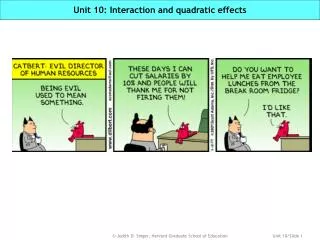
5. Examples of Statistical Interactions Statistical interaction When the effect of one predictor differs by the level of another predictor Brain Functioning Teens Adults Hours after 8 pm Tax season Interest level Non-tax season Hours watching documentaries Dilbert cartoon on Unit 10 Cover: Effect of 10% salary reduction on employee morale differs by the economic climate.

6. Example: Does the effect of father presence differ by paternal behavior? Child ASB 33.00 30.00 27.00 24.00 21.00 18.00 15.00 12.00 -25 0 25 50 75 100 125 % of Child Life that Father is Resident n =1,116 children, followed from birth through childhood “[The goal] was to determine whether the effects of father presence were uniform across families. Our hypothesis was that the fathers’ antisocial behavior would moderate the effect of father presence, such that when a father engaged in low levels of antisocial behavior, the less time he resided with his children the more behavior problems his children would have. In contrast, when a father engaged in high levels of antisocial behavior, the more time he resided with his children, the more behavior problems his children would have” Source: Jaffee, SR, Moffitt, TE, Caspi, A, & Taylor, A (2003). Life with (or without) father: The benefits of living with two biological parents depend on the father’s antisocial behavior. Child Development, 74(1) 109-126. High Antisocial Father (85th %ile) “Figure 1 plots the interaction and shows the simple slopes for the effect of father presence on child antisocial behavior at three values of the fathers’ antisocial behavior distribution (15th, 50th, and 85th percentiles). The figure shows that at low and median levels of fathers’ antisocial behavior, father presence was negatively associated with children’s antisocial behavior, such that the longer a father resided with his child, the less antisocial behavior the child had. However, at high levels of fathers’ antisocial behavior, father presence was positively associated with child antisocial behavior, such that the longer a father resided with his child, the more antisocial behavior he had.” Mid Antisocial Father (50th %ile) Low Antisocial Father (15th %ile)

7. Interactions are prevalent in social science research • (1) Interactions form the basis for several quasi-experimental analytic methods: • Regression discontinuity design (e.g., Gormley et al., 2005, on Universal Pre-K in Oklahoma) • Difference-in-Differences (e.g., Dynarski, 2003, on College Financial Aid). (2) Interactions between variables are common in the research literature. Not surprisingly, especially in education, the effect of one variable differs by levels of another Potkay & Potkay, 1984 How much readers identify with cartoon characters of different genders differs by the gender of individual (interaction of gender of cartoon character and gender of reader). Castleman et al., 2009 (preliminary) Relationship between ELA test scores and college enrollment is positive for traditional public school students, but there is no relationship for charter school students (interaction of test scores and charter schooling). Johnson & Birkeland, 2009 The experiences of teachers in alternative certification programs depend on characteristics of the individual, the program, and their school (interaction of school, program, and person). Reardon et al., 2009 The effect of failing the mathematics high school exit examination in CA is bigger for students who also failed the English language arts examination (interaction of math and ELA test performance).

8. What is a statistical interaction?And how is it different from the effects that we’ve modeled so far? Child ASB High Antisocial Father Mid Antisocial Father Low Antisocial Father Loge(Price) % of Child Life that Father is Resident Burgundy Bordeaux Rhone Languedoc Vintage Models to date: The fitted lines have been parallel New model: The fitted lines are not parallel Main effects model The fitted lines are parallel because the main effects model assumes that the effect of each predictor is identical regardless of the values of all other predictors in the model. This model assumes that we can describe the effect of any predictor holding all other predictors in the model constant at any particular value. Statistical interaction model The fitted lines are NOT assumed to be parallel because the interaction model allows the effect of each predictor to differ by values of all other predictors in the model. This model assumes that we cannot simply describe the effect of any predictor holding all other predictors in the model constant because the effect may differ according to those values.

9. Two types of statistical interactions: Ordinal and Disordinal Lung Cancer Activity Level Non ADHD ADHD Asbestos Exposure Dose of Ritalin Ordinal interaction The direction of each predictor’s effect is consistent across levels of the other predictor, but its magnitudediffers Disordinal interaction The directionof the effect of one predictor differs across levels of the other predictor Smokers Non-smokers Q: If the lines in an ordinal interaction aren’t parallel, won’t they eventually cross, making all ordinal interactions disordinal? Whether ordinal or disordinal, all interactions share a common feature —non parallel lines— So the test that detects a statistical interaction is often called a test of parallelism Always graph your fitted model within the range of the data.

10. Introducing the case study: Sector differences in college graduation rates April 23, 2006   • Questions you might want to ask: • Okay, there’s a difference by sector, but are all types of private colleges equally effective at graduating a larger proportion of their entering freshmen? • From our earlier work, we might ask: Does this public-private sector differential change if we control statistically for other factors associated with graduation rates? • E.g., if we control for the quality of the student body & amount of financial aid, does the public-private gap change? • Today, we’ll learn how to ask: Does the public/private sectordifferentialdiffer by the levels of other school characteristics? • E.g,. are selective public schools (like UC Berkeley) similar to other public schools or are they more like private schools? • In other words, does the “effect” of sector differ at different values of these other predictors? • In other words, might there be a statistical interaction between sector and other predictors of college graduation rates?

11. Data to address these research questions Source: Scott, M, Bailey, T, & Kienzl, G (2006). Relative success: Determinants of college graduation rates in public and private colleges in the US, Research in Higher Education, 47(1), 249-279 ID Name PctGrad Public SAT SATDiff FinAid 1 ABILENE CHRISTIAN UNIVERSITY 53.0000 0 11.00 3.20 75 2 ACADEMY OF THE NEW CHURCH 55.4425 0 11.70 3.20 62 3 ADAMS STATE COLLEGE 43.0000 1 10.10 3.10 84 4 ADELPHI UNIVERSITY 46.9892 0 10.20 2.90 78 5 ADRIAN COLLEGE 46.0000 0 9.70 1.80 85 6 AGNES SCOTT COLLEGE 61.0000 0 11.90 2.80 94 7 ALABAMA A&M UNIVERSITY 34.0000 1 8.40 2.30 60 8 ALABAMA STATE UNIVERSITY 24.1702 1 7.50 2.00 90 9 ALASKA BIBLE COLLEGE 35.5643 0 10.10 5.00 67 10 ALASKA PACIFIC UNIVERSITY 37.1983 0 10.40 3.30 69 11 ALBANY COLLEGE OF PHARMACY 76.0000 0 11.10 1.60 79 12 ALBANY STATE COLLEGE 33.4602 1 8.00 1.50 88 13 ALBERTSON COLLEGE OF IDAHO 66.4433 0 10.40 1.00 80 14 ALBERTUS MAGNUS COLLEGE 44.0000 0 10.10 .60 74 15 ALBION COLLEGE 68.0000 0 11.30 1.60 80 16 ALBRIGHT COLLEGE 63.0000 0 12.00 2.00 67 17 ALCORN STATE UNIVERSITY 34.0000 1 9.70 4.10 92 18 ALDERSON BROADDUS COLLEGE 44.8082 0 11.00 3.00 91 19 ALFRED UNIVERSITY 67.0000 0 12.30 2.40 90 Histogram of PctGRAD # Boxplot 97.5+*** 11 | .****** 21 | .******** 30 | .********** 37 | .************** 55 | .********************* 83 | .**************************** 111 | .******************************* 121 +-----+ .************************************ 143 | | 52.5+****************************************** 168 | | .***************************************** 162 *--+--* .***************************************** 161 | | .************************************** 151 +-----+ .************************************ 142 | .************************** 102 | .********************* 82 | .****** 22 | .**** 15 | 7.5+* 4 | ----+----+----+----+----+----+----+----+-- * may represent up to 4 counts RQ 2: Do the effects of these other predictors differ by sector? RQ 1: Besides sector, what else predicts college graduation rates? n = 1621 RQ 2: Does the effect of sector differ by these other predictors? RQ 2: In other words, is there an interaction? Does school selectivity or financial aid have a different effect in public schools than it does in private schools?

12. Predicting college graduation rates (a first look…) relatively uncorrelated (although the r’s of |.07| are stat sig because of the large sample size) These 3 predictors are higher in schools with stronger student bodies Graduation rates are Pearson Correlation Coefficients, N = 1621 Prob > |r| under H0: Rho=0 PctGrad SAT SATDiff FinAid Public PctGrad 1.00000 0.75150 -0.26589 0.02812 -0.24014 <.0001 <.0001 0.2578 <.0001 SAT 0.75150 1.00000 0.00533 -0.07362 -0.10078 <.0001 0.8302 0.0030 <.0001 SATDiff -0.26589 0.00533 1.00000 0.07059 -0.00402 <.0001 0.8302 0.0045 0.8715 FinAid 0.02812 -0.07362 0.07059 1.00000 -0.45010 0.2578 0.0030 0.0045 <.0001 Public -0.24014 -0.10078 -0.00402 -0.45010 1.00000 <.0001 <.0001 0.8715 <.0001 r = 0.75*** Graduation rates are lower in schools with more heterogeneous student bodies Financial aid appears to have no relationship with PctGrad (uncontrolled at least) In contrast to private colleges, public colleges: r = -0.27*** • Have lower graduation rates • Have somewhat less strong student bodies • Are indistinguishable in terms of student body heterogeneity • Have smaller percentages of students on financial aid We already know how to address RQ1 about the predictors’ effects, but how do we address RQ2 about the statistical interaction? r = 0.03 (ns)

13. How do we test for the presence of a statistical interaction? There’s an easy, three-step process! Step 1: Create a cross-product term, which is literally the product of the two predictors whose interaction you want to test (e.g, PSAT=SAT*Public) (NOTE: In your data step in SAS, just write PSAT = SAT*public;) ID Name PctGrad Public SAT PSAT 1 ABILENE CHRISTIAN UNIVERSITY 53.0000 0 11.00 0 2 ACADEMY OF THE NEW CHURCH 55.4425 0 11.70 0 3 ADAMS STATE COLLEGE 43.0000 1 10.10 10.10 4 ADELPHI UNIVERSITY 46.9892 0 10.20 0 5 ADRIAN COLLEGE 46.0000 0 9.70 0 6 AGNES SCOTT COLLEGE 61.0000 0 11.90 0 7 ALABAMA A&M UNIVERSITY 34.0000 1 8.40 8.40 8 ALABAMA STATE UNIVERSITY 24.1702 1 7.50 7.50 9 ALASKA BIBLE COLLEGE 35.5643 0 10.10 0 10 ALASKA PACIFIC UNIVERSITY 37.1983 0 10.40 0 11 ALBANY COLLEGE OF PHARMACY 76.0000 0 11.10 0 12 ALBANY STATE COLLEGE 33.4602 1 8.00 8.00 13 ALBERTSON COLLEGE OF IDAHO 66.4433 0 10.40 0 14 ALBERTUS MAGNUS COLLEGE 44.0000 0 10.10 0 15 ALBION COLLEGE 68.0000 0 11.30 0 16 ALBRIGHT COLLEGE 63.0000 0 12.00 0 17 ALCORN STATE UNIVERSITY 34.0000 1 9.70 9.70 18 ALDERSON BROADDUS COLLEGE 44.8082 0 11.00 0 19 ALFRED UNIVERSITY 67.0000 0 12.30 0 Step 2: Include thecross-product in a MR model that also includes the constituent main effects (NOTE: You should always include the main effects) Step 3: Test H0: cross-product = 0 If the individual t-test rejects H0, the two predictors interact; if not, there is no statistical interaction between these two predictors NOTE on terminology: Main Effects Cross-Product Term

14. Remembering dichotomous predictors: Main effects model Our simple, main effects model: Private Public

15. Why does a cross-product term tell us about a statistical interaction? Note the inclusion of main effects Our interaction model with cross-product term The parameter estimate for the interaction term tells us how much steeper the slope on SAT is for public schools than for private schools Private 1 Public

16. Is there a statistically significant interaction between SECTOR and SAT?Comparing main effects and interaction models We can reject the null hypothesis that all predictors in each model have no effect Reasonably high R2 in both models (although the interaction model seems only trivially better than the main effects model) Main effects model Sum of Mean Source DF Squares Square F Value Pr > F Model 2 311744 155872 1174.11 <.0001 Error 1618 214802 132.75777 Corrected Total 1620 526546 Root MSE 11.52206 R-Square 0.5921 Dependent Mean 49.72992 Adj R-Sq 0.5916 Coeff Var 23.16926 Parameter Standard Variable DF Estimate Error t Value Pr > |t| Intercept 1 -45.38289 2.16172 -20.99 <.0001 SAT 1 9.23804 0.20066 46.04 <.0001 Public 1 -6.33366 0.60861 -10.41 <.0001 Interaction effect model Sum of Mean Source DF Squares Square F Value Pr > F Model 3 312657 104219 787.89 <.0001 Error 1617 213889 132.27538 Corrected Total 1620 526546 Root MSE 11.50110 R-Square 0.5938 Dependent Mean 49.72992 Adj R-Sq 0.5930 Coeff Var 23.12713 Parameter Standard Variable DF Estimate Error t Value Pr > |t| Intercept 1 -41.32250 2.65428 -15.57 <.0001 SAT 1 8.85605 0.24751 35.78 <.0001 Public 1 -17.87644 4.43583 -4.03 <.0001 PSAT 1 1.10674 0.42131 2.63 0.0087 Both SAT and Public each have statistically significant main effects There is a statistically significant interaction between SAT and Public (in this simple uncontrolled model) The main effects assumption doesn’t hold: The effect of SAT scores differs by sector CAUTION: Do NOT try to interpret the main effects by themselves Built in assumptions: The effects of SAT are identical in private and public colleges and the private-public differential is identical across the full range of SAT scores The public/private differential differs by selectivity of school. Until we “do the math” we don’t know how it differs, we just know that it does.

17. Graphing and interpreting a model with a statistical interaction Private Public 1.11, the coefficient for the cross-product, is the increment to the slope (“effect” of SAT)in public schools -17.88, the coefficient for Public, assesses the public/private difference when SAT=0 (not interesting here) -41.32, the y-intercept, is the predicted grad rate in private schools with SAT=0 (rarely interpreted) 8.86, the coefficient for SAT, is the slope (“effect” of SAT) when Public=0 (in private schools)

18. All interaction effects can be summarized in (at least) two different waysdepending on which predictor you choose to focus upon Child ASB High Antisocial Father PctGrad Mid Antisocial Father Low Antisocial Father % of Child Life that Father is Resident 75th %ile of SAT (in 100s) Interpretation #1 The effect of SAT scores differs by sector The effect is larger (the slope is steeper) among public colleges than among private colleges Interpretation #1 The effect of father presence differs by levels of paternal antisocial behavior The effect is positive for low antisocial fathers and negative for high antisocial fathers Interpretation #2 The effect of sector (the public/private differential) differs by SAT scores The weaker the student body, the larger the differential; when the student body of a school is very strong, there is no differential Interpretation #2 The effect of paternal antisocial behavior differs by the %age of a child’s life that the father is resident The more time the child lives with the father, the larger the effect

19. Comparing the interaction model to separate models fit within SECTOR Why can’t we just fit separate models for public and private schools? Effect of SAT in private colleges Public=0 Number of Observations Used 1075 Root MSE 11.82350 R-Square 0.5303 Dependent Mean 52.81446 Adj R-Sq 0.5298 Coeff Var 22.38687 Parameter Estimates Parameter Standard Variable DF Estimate Error t Value Pr > |t| Intercept 1 -41.32250 2.72868 -15.14 <.0001 SAT 1 8.85606 0.25445 34.80 <.0001 Interaction effect model Number of Observations Used 1621 Root MSE 11.50110 R-Square 0.5938 Dependent Mean 49.72992 Adj R-Sq 0.5930 Coeff Var 23.12713 Parameter Standard Variable DF Estimate Error t Value Pr > |t| Intercept 1 -41.32250 2.65428 -15.57 <.0001 SAT 1 8.85605 0.24751 35.78 <.0001 Public 1 -17.87644 4.43583 -4.03 <.0001 PSAT 1 1.10674 0.42131 2.63 0.0087 Effect of SAT in public colleges Public=1 Number of Observations Used 546 Root MSE 10.83712 R-Square 0.6387 Dependent Mean 43.65689 Adj R-Sq 0.6381 Coeff Var 24.82338 Parameter Estimates Parameter Standard Variable DF Estimate Error t Value Pr > |t| Intercept 1 -59.19894 3.34888 -17.68 <.0001 SAT 1 9.96280 0.32125 31.01 <.0001 • Advantages of interaction models • Interaction models can be fit whether the predictors are dichotomous or continuous • Interaction models provide an easy statistical test of whether the slopes differ across groups (or across levels of a continuous predictor). • Interaction models keep the sample intact (you don’t need to break it down into many different groups).

20. Are there interactions between the other predictors and SECTOR? PctGrad PctGrad IQR of SAT (in 100s) % students on financial aid What’s the effect of heterogeneity (SATDiff) in private schools? What’s the effect of heterogeneity (SATDiff) in public schools? How does the effect of heterogeneitydiffer by sector? Heterogeneity has a larger effect in public than it does in private schools How does the effect of sector differ by heterogeneity? The more homogeneous the student body, the smaller the sector differential What’s the effect of financial aid in private schools? What’s the effect of financial aid in public schools? How does the effect of financial aid differ by sector? If we test each interaction on its own, not controlling for any other predictors (or interactions), all three tests reject the null hypothesis (!) The effect of FinAid is positive in public schools and negative in private ones How does the effect of sector differ by financial aid? The more financial aid offered, the smaller the sector differential

21. Do the interactions remain when we control for all main effects? These equations result from substituting in the values for PUBLIC (0=private, 1=public) From Model D (the main effects model) we conclude that all three main effects—SAT, SATDiff and FinAid—are statistically significant and should be included in our model; controlling for these three, there’s a main effect of SECTOR From Model E we conclude that when we control statistically for the main effects of SATDiff and FinAid, there is no interaction between SAT and SECTOR. Thus, we do not need to keep the cross-product term (PUBLIC*SAT) in our model. From Model F we conclude that when we control statistically for the main effects of SAT and FinAid, there is no interaction between SATdiff and SECTOR. Thus, we do not need to keep the cross-product term (PUBLIC*SATDiff) in our model. From Model G we conclude that when we control statistically for the main effects of SAT and SATDiff, the interaction between FinAid and SECTOR persists What about the n.s. main effect of FinAid in Model G? The effect of FinAid is non-significant in Private schools. But…..Never delete main effects that are components of a statistically significant interaction EVEN IF THEY ARE NON-SIGNFICANT! NEVER!* *or at least not yet

22. How might we summarize our findings, including the interaction? SATdiff 10th & 90th %iles = 1.7 and 3.4 SAT 10th & 90th %iles = 8.8 and 12.3 PctGrad 90.00 70.00 50.00 30.00 10.00 0 25 50 75 100 % students on financial aid Note: Remember what our variables mean substantively What’s the effect of SAT scores? Controlling for SAT homogeneity, financial aid and sector, the higher the 75th %ile of SAT scores, the higher the graduation rate Very strong SAT scores What’s the effect of SAT homogeneity? Private Homogeneous scores The more homogeneous the SAT scores, the higher the graduation rate (holding constant the 75th%ile of SAT scores, financial aid and sector) Public Private Heterogeneous scores Public What’s the effect of Financial Aid? Controlling for SAT scores (both 75th %ile and IQR) the relationship between financial aid and graduation rates differs by SECTOR. In private schools, AID has almost no effect; in public schools, the larger the %age of students receiving aid, the higher the graduation rate (seen in slope of lines) Very weak SAT scores Private Homogeneous scores Public Private Heterogeneous scores Public What’s the effect of SECTOR? Controlling for SAT scores (both 75th %ile and IQR) the effect of SECTOR differs by financial aid. In schools that provide most students with aid, there is no sector differential; the lower the %age of students receiving aid, the larger the public/private differential

23. Now that we know about interactions, what about the Ed School data? Were those lines really parallel? = Large Schools = Medium Schools = Small Schools × = School L2Doc GRE L2DocGRE Harvard 5.90689 6.625 39.1332 UCLA 5.72792 5.780 33.1074 Stanford 5.24793 6.775 35.5547 TC 7.59246 6.045 45.8964 Vanderbilt 4.45943 6.605 29.4545 Northwestern 3.32193 6.770 22.4895 Berkeley 5.42626 6.050 32.8289 Penn 5.93074 6.040 35.8217 Michigan 5.24793 6.090 31.9599 Madison 6.72792 5.800 39.0219 NYU 6.80735 5.960 40.5718 Large Medium Small Interaction effect model R2=66.8% Parameter Standard Variable DF Estimate Error t Value Pr > |t| Intercept 1 441.63946 198.90350 2.22 0.0292 PctDoc 1 0.74971 0.18698 4.01 0.0001 L2Doc 1 -94.53164 40.04790 -2.36 0.0206 GRE 1 -32.93383 35.38194 -0.93 0.3547 L2DocGRE 1 18.93133 7.10577 2.66 0.0093 Should we do anything about the main effect of GRE? NO!

24. Interpreting and displaying an interaction between continuous predictors Peer Rating 500 450 400 350 300 250 4.5 5.0 5.5 6.0 6.5 7.0 Mean GRE Mean GRE Scores = on the x-axis PctDoc = 38.20 (sample mean) Small: L2Doc = 4 (NDoc=16) Medium: L2Doc = 5 (NDoc=32) Large: L2Doc = 6 (NDoc=64) • In our main effects model, the lines: • Have different intercepts, but were a constant distance apart (distance = controlled effect of L2DOC) • Have the same slope (slope = controlled effect of GRE) • In our interaction effects model, the lines: • Have different intercepts and are not a constant distance apart (controlled effect of L2DOC still seen in distance between lines, but it varies at different levels of GRE) • Have different slopes (controlled effect of GRE still seen in the slope, but it varies at different levels of L2DOC) Large Medium Small

25. Interpreting and displaying an interaction between continuous predictors Peer Rating 500 450 400 350 300 250 4.5 5.0 5.5 6.0 6.5 7.0 Mean GRE Large Medium Small What’s the effect of program size? What’s the effect of mean GRE scores? • Holding PctDoc constant,the effect of program size differs by mean GRE score(distance between lines). • In schools with low mean GREs, there’s virtually no effect of program size; the higher a school’s mean GRE scores, the larger the effect of program size. • For example, when mean GRE = 500, a doubling of size is associated with a 0.12 difference in peer ratings, whereas when mean GRE = 600, a doubling of size is associated with a 19.05 difference in ratings. • Holding PctDoc constant, the effect of mean GRE score differs by department size(slope of the lines). • The larger the school, the larger the effect of GRE scores. • For example, among small schools (L2Doc = 4) a difference of 100 points in mean GRE is associated with a 42.8 point in peer ratings, whereas among large schools (L2Doc = 6), the same 100-point difference in mean GRE scores is associated with a 80.65 difference in peer rating.

26. and (2) Don’t extrapolate beyond the range of the data Caveats: (1) Don’t confuse interaction with correlation Child ASB High Antisocial Father Mid Antisocial Father Low Antisocial Father % of Child Life that Father is Resident Predictors are not correlated Predictors are correlated Predictors do not interact Predictors do interact Caveat 1 Interaction The effect of X1 differs by levels of X2 Correlation X1 and X2 are associated SAT and SATDiff are not correlated, and although not documented here, they do not interact in predicting graduation rates SAT verbal and math are correlated but they do not interact when predicting college achievement • Correlation does not imply interaction • Just because two predictors are correlated doesn’t suggest anything about whether they might interact. • The question to ask is whether there’s reason to hypothesize that the effect of one predictor might differ according to levels of another predictor. SATDiff and Public are not correlated, but they do interact in predicting grad rates (not controlling for other predictors) Financial aid and Public are correlated and they do interact in predicting graduation rates Caveat 2 Of course this reversal makes no sense: it’s outside the range of our data and we shouldn’t be predicting there!

27. A very special interaction: A predictor can interact with itself! Y X All quadratics are non-monotonic—they both rise and fall (or fall and rise) Satisfaction Q: What if the effect of a given predictor differed by levels of that very predictor—the “effect of X” differed by levels of X? Quadratic model We allow a predictor’s effect to differ according to levels of that predictor. The test on 2 provides a test of whether the quadratic term (model) is necessary Number of Jellybeans Eaten At low levels of X, the relationship between Y and X is relatively steep and positive At high levels of X, the relationship between Y and X is relatively steep and negative At moderate levels of X, the relationship between Y and X is quite flat (almost no relationship)

28. You’re only interested in the shape of a quadratic within the range of X Y Y X X Source: Finch, BK (2003). Socioeconomic gradients and low birth-weight: Empirical and policy considerations. Health Services Research, 38(6), 1819-1841. “Research has argued that the shape of the relationship between SES and health is actually curvilinear such that there are decreasing returns to health as SES increases. When you’re poor, $1000 has a bigger effect than when you’re rich Thus, quadratics are another tool we can use to transform our data and fit non-linear relationships

29. Wine ratings redux: Does quality (or at least ratings) matter? Loge(price) Residuals from linear regression on Rating Rating The effect of rating on price is small when ratings are low and high when ratings are high ID Lprice Rating Rating2 1 2.54721 7 49 3 2.58238 6 36 31 3.29584 8 64 33 3.33831 8 64 35 3.39881 7 49 50 3.70658 10 100 57 3.85167 10 100 58 3.91488 9 81 60 4.19570 11 121 61 2.64820 1 1 66 3.00285 5 25 67 3.00498 4 16 Rating2 = Rating*Rating The REG Procedure Dependent Variable: Lprice Root MSE 0.30576 R-Square 0.5276 Dependent Mean 3.06102 Adj R-Sq 0.5190 Coeff Var 9.98886 Parameter Estimates Parameter Standard Variable DF Estimate Error t Value Pr > |t| Intercept 1 2.50664 0.26885 9.32 <.0001 Rating 1 -0.03372 0.07640 -0.44 0.6598 Rating2 1 0.01461 0.00537 2.72 0.0075 The t-statistic for Rating2 indicates that the linear term is not sufficient. We need to include Rating2 in our model.

30. Does the effect of Rating remain quadratic after controlling for Region and Vintage? Loge(price) Burgundy Bordeaux Predicted Log Price Rhone Languedoc Rating Languedoc Burgundy Bordeaux Rhone 1 2.27177 2.99557 2.4999 2.44667 .. .. .. .. .. 4 2.44196 3.16576 2.67009 2.61686 5 2.54177 3.26557 2.7699 2.71667 .. .. .. .. .. 10 3.36392 4.08772 3.59205 3.53882 11 3.59297 4.31677 3.8211 3.76787 Rating Actual price The REG Procedure Model: MODEL1 Dependent Variable: Lprice Root MSE 0.21313 R-Square 0.7788 Dependent Mean 3.06102 Adj R-Sq 0.7663 Coeff Var 6.96281 Parameter Estimates Parameter Standard Variable DF Estimate Error t Value Pr > |t| Intercept 1 2.45448 0.20852 11.77 <.0001 Burgundy 1 0.72380 0.08279 8.74 <.0001 Bordeaux 1 0.22813 0.05701 4.00 0.0001 Rhone 1 0.17490 0.06183 2.83 0.0056 Year 1 -0.09673 0.02136 -4.53 <.0001 Rating 1 0.00288 0.05518 0.05 0.9584 Rating2 1 0.01077 0.00380 2.83 0.0055 $148.41 +0.23 $54.60 +0.10 $20.09 Set YEAR at its mean = 2.04 $7.39 After controlling for linear vintage and quadratic ratings, which regions are significantly different? The effect of 1-unit difference in rating is smaller when ratings are lower… +0.10 … and bigger when ratings are higher. +0.23

31. Bonferroni multiple comparisons of REGION means (controlling for RATING, RATING2 and VINTAGE) The GLM Procedure Least Squares Means Adjustment for Multiple Comparisons: Bonferroni Lprice LSMEAN Region LSMEAN Number 1 3.58861155 1 2 3.09294691 2 3 3.03971063 3 4 2.86481291 4 Least Squares Means for Effect Region t for H0: LSMean(i)=LSMean(j) / Pr > |t| Dependent Variable: Lprice i/j 1 2 3 4 1 5.93396 6.207648 8.742802 <.0001 <.0001 <.0001 2 -5.93396 0.942968 4.001843 <.0001 1.0000 0.0007 3 -6.20765 -0.94297 2.828796 <.0001 1.0000 0.0335 4 -8.7428 -4.00184 -2.8288 <.0001 0.0007 0.0335 Burgundy Bordeaux Rhone Languedoc Bordeaux and the Rhone are indistinguishable after controlling for linear vintage and the quadratic effect of rating Burgundy Bordeaux Rhone Languedoc Burgundy is significantly more expensive than all other regions after controlling for linear vintage and the quadratic effect of rating Burgundy Bordeaux Rhone Languedoc The Languedoc remains significantly less expensive than all other regions, after controlling for linear vintage and the quadratic effect of rating

32. Hypothesizing the existence of quadratic effects: A recent example

33. What’s the big takeaway from this unit? • Statistical interactions are an important type of effect • An interaction tells us that the effect of one predictor varies by levels of another • Sometimes the magnitude of an effect will vary; other times the direction of an effect will vary • The standard regression model, which initially assumes that there are no interactions, can be easily modified to accommodate their presence • Many substantive theories suggest that effects will be interactive • You test for a statistical interaction by adding a cross-product term • The cross-product is literally the product of the two constituent variables • If it is significant in a model that also includes the constituent main effects, you know that the two predictors interact. And never remove the main effects • Graph out the fitted model to ensure correct interpretation. • Predictors can interact with themselves! • Quadratic models provide a flexible strategy for fitting nonlinear models, especially those that can’t be linearized by taking logarithms • Substantive theories often suggest that a predictor’s effect may be quadratic • You test for the presence of a quadratic effect and include it in a regression model using the same strategy used to include interaction effects

34. Appendix: Annotated PC-SAS Code for Interactions and Quadratic Effects The data step here is used to create cross-product terms, literally the product of the two variables whose interaction you want to test. It is often helpful to add a where statementto a proc print, because it tells SAS to print out only a subset of the data (here, IDs 1 – 19). This can save reams of paper! *------------------------------------------------------------------* Listing data on observations 1-19 for inspection *------------------------------------------------------------------*; procprint data=one; where 1 <= id <= 19; var id name pctgrad public sat satdiff finaid; run; The data stepis also the place to create quadratic terms. You can either multiply a variable by itself (i.e., rating2=rating*rating) or more easily just raise the variable to the second power (as done in this code). Wine Analysis data one; infile "m:\datasets\wine.txt"; input ID 1-3 Price 5-16 Region 19 Area $ 21-31 Year 34 Vintage $ 38-44 Rating 48-51; Rating2 = rating**2; Gradrate Analysis *-------------------------------------------------------------------* Input Gradrate data and name variables in dataset Create interaction terms PSAT, PSATDIFF, & PFINAID *------------------------------------------------------------------*; data one; infile "m:\datasets\gradrate.txt"; input ID 1-4 Name $ 7-47 PctGrad 50-61 Public 64 SAT 67-70 SATdiff 73-76 FinAid 78-80; PSAT=public*sat; PSATDiff=public*satdiff; PFinAid=Public*FinAid;

35. Glossary terms included in Unit 10 • Interactions (ordinal and disordinal) • Quadratics

36. Unit 6, Slide 17: Understanding the fitted MR model algebraically & graphically 3 4 5 6 7 Graphically Return to the plot from before Algebraically Plug in different values of L2Doc Controlled effect of GRE can be seen in the commonslope (63.32) of these lines 4.75 -(-10.59) 15.34 -10.59 -(-25.93) 15.34 -25.93 -(-41.27) 15.34 Controlled effect of L2Doc can be seen in the common distance (15.34) between these lines

37. Appendix: Visualizing a statistical interaction PEER The twist in the “plane” allows the relationship (slope) between PEER and GRE to vary at different values of L2DOC. We can see this twist by looking at the fitted regression “plane” in our 3D view from two different angles. L2DOC = 7 L2DOC = 3 PEER L2DOC = 7 L2DOC = 3