Download
1 / 47
500 likes | 826 Views
Spatial e cology and demography of eastern coyotes in western Virginia. Dana Morin Working Plan Presentation. Introduction. Eastern range expansion of coyotes. Mike St Germain. Parker 1995, Animal Planet, bioweb. Introduction. Eastern range expansion of coyotes. Mike St Germain.

E N D
Spatial ecology and demography of eastern coyotes in western Virginia Dana Morin Working Plan Presentation
Introduction • Eastern range expansion of coyotes Mike St Germain Parker 1995, Animal Planet, bioweb
Introduction • Eastern range expansion of coyotes Mike St Germain Parker 1995
Introduction • Eastern range expansion of coyotes Mike St Germain Parker 1995
Introduction • Eastern range expansion of coyotes Mike St Germain Parker 1995
Introduction • Coyotes in Virginia
Human-wildlife conflicts • Livestock and agricultural losses • Tomsa and Forbes 1989 • Wooding and Hardisky 1990 • Witmer and Hayden 1991 • Witmer et al. 1993 • Armstrong and Walters 1995 • NASS 1999 • Main et al. 2002 • Gompper 2002a • Houben 2004 USDA
Human-wildlife conflicts • Perceived threat to humans and pets • Bider and Weil 1984 • Chambers 1987 • Billodeaux 2007 KnoxNews Joseph Hinton
Potential conflicts • Negative impacts to prey species? • Negative impact: • Cook et al. 1971, Stout 1982, Hamlin et al. 1984, Messier et al. 1986, Chambers 1987, Blanton and Hill 1989, NASS 1999, Ballard and Whitlaw 1999, Houben 2004, Staller et al. 2005, Saalfeld and Ditchkoff 2007, Kilgo et al. 2010 • No impact: • But see also: Ozoga and Harger 1966, Westmoreland and Woolf 1981, Decker et al. 1992, Wagner and Hill 1994, Crete and Derosier 1995, Cox 2003, Bumann and Stauffer 2002 Mark Taylor (Roanoke.com)
Potential conflicts • Negative impacts to prey species? • Negative impact: • Cook et al. 1971, Stout 1982, Hamlin et al. 1984, Messier et al. 1986, Chambers 1987, Blanton and Hill 1989, NASS 1999, Ballard and Whitlaw 1999, Houben 2004, Staller et al. 2005, Saalfeld and Ditchkoff 2007, Kilgo et al. 2010 • No impact: • But see also: Ozoga and Harger 1966, Westmoreland and Woolf 1981, Decker et al. 1992, Wagner and Hill 1994, Crete and Derosier 1995, Cox 2003, Bumann and Stauffer 2002 Mark Taylor (Roanoke.com)
Plasticity • Behavioral and phenotypic plasticity • Hybridization • Natural selection western coyote (Michael Anguiano) eastern coyote (Joseph Hinton)
Study Area Rockingham Bath Highland Augusta
Objectives • Spatial Ecology • Movement patterns and home range • Habitat selection • Demography • Densities • Population growth rates • Social structure
Objectives • Spatial Ecology • Movement patterns and home range • Habitat selection • Demography • Densities • Population growth rates • Social structure
Objectives • Population responses to anthropogenic effects • Development of population simulation model
Objectives • Population responses to anthropogenic effects • Development of population simulation model
General Methods • Trapping and fitting with satellite collars • Scat transects with genetic identification to individual • Extraction of GIS landscape/land use variables • Incorporation of prey variables (deer, small mammals, vegetation)
Objective 1 - methods • Home range and habitat selection • Trapping with padded foothold • 12 satellite collars each year on trapped individuals • 6 in spring • 6 in fall • 5 daily locations • plus rotation of fine temporal scale locations
Objective 1 – home range methods • Kernel density methods • 95% fixed kernel home range (Worton 1989) • 50% fixed kernel core areas • Home range overlap • At 95% and 50% levels • (Schrecengost et al. 2009) • Maximum dispersal distances
Objective 1 – home range expectations • Large amount in variation (1.8 km2 - 122.9 km2) • Typically larger in forested areas than rural areas • More seasonal variation in forested areas • Substantial home range overlap between group members, little overlap between groups Post 1975, Ford 1983, Smith 1984, Sumner 1984, Harrison 1986, Priest 1986, Babb 1988, Person 1988, Morton 1989, Parker and Maxwell 1989, Crawford 1992, Holzman et al. 1992, Brundige 1993, Edwards 1996, Lovell 1996, Kendrot 1998, Eastman 2000, Way 2000, Crete et al. 2001, Bogan 2004, Atwood and Weeks 2002a, Atwood and Weeks 2002b, Gehrt 2007, Gehrt et al. 2009, Schrecengost et al. 2009
Objective 1 – habitat selection methods • Hierarchical Approach (Oehler and Litvaitis 1996) • Landscape and home range level (Boisjoly et al. 2010) • Presence only: Compare confirmed fine scale locations to available habitats • Detection/nondetection: “Occupancy” models (MacKenzie 2005)in program PRESENCE at habitat scale
Objective 1 – habitat selection expectations • early successional habitat > mature forest stands > agricultural > suburban/urban Crossett 1990, Kendrot 1998, Dumond et al. 2001, Gosselink et al. 2003, Bogan 2004, Atwood and Weeks 2002a, Atwood et al. 2004, Gehrt 2007, Kays et al. 2008, Page 2010, Weckel et al. 2010
Objective 1 – habitat selection expectations • Vary with season, land use, and food availability Post 1975, Litvaitis and Harrison 1989, Lovell 1996, Chamberlain 1999, Priest 1986, Parker and Maxwell 1989, Person and Hirth 1991, Holzman et al. 1992, Brundige 1993, Stupakoff 1994, Oehler and Litvaitis 1996, Crete and Lariviere 2003, Thibault and Oullet 2005, Billodeaux 2007
Objective 2 – Demography methods • Scat transects • sampling model dependent • Genotyping faeces to individual • Capture-Mark-Recapture Models (CMR)
Objective 2 – Density methods • 2 large study grids • 200 km2 (3-4 x home range - Maffei and Noss 2008) • Bath County (forested) • Rockingham County (forest-rural interface)
Objective 2 – Density methods • 2 large study grids • 200 km2 (3-4 x home range - Maffei and Noss 2008) • Bath County (forested) • Rockingham County (forest-rural interface) 200 km2
Objective 2 – Density methods • 2 large study grids • 200 km2(3-4 x home range - Maffei and Noss 2008) • Bath County (forested) • Rockingham County (forest-rural interface) 200 km2 200 km2
Objective 2 – Density methods • Scat transects • Standardized total transect length per grid cell • Transects cleared and scat collected 1 month later
Objective 2 – Density methods • Spatially Explicit Capture-Recapture models (SECR) • Produce density estimate and effective sampling area • SPACECAP (Royle and Young 2008) • DENSITY (Efford 2004) 200 km2 200 km2
Objective 2 – Density expectations • Large amount of variation: • Season • Available food resources • Latitude • Habitat • Highest post-whelping • Greater to the south • Median: 0.5/ km2 (Sumner 1984, Parker 1995, Clark 1972, Stoddart and Knowlton 1983, Gese et al, 1989, Parker 1995, Knowlton and Gese 1995, Rose and Polis 1998, Patterson et al. 1998, Fisher 1977, Smith 1984, Priest 1986, Chambers 1987, Blanton 1988, Babb and Kennedy 1989, Stephenson and Kennedy 1993, Samson and Crete 1997, Lloyd 1998, Patterson and Messier 2001, Richer et al. 2002, Kays et al. 2008)
Objective 2 – Population growth methods • Estimate changes in abundance over time • Pradel reverse-time models (open populations) 200 km2 200 km2
Objective 2 – Population growth methods • Subsample Pradel sites • 2 primary surveys/year (summer and winter) 200 km2 200 km2
Objective 2 – Population growth methods s5 s1 s2 s3 s4 s6 Summer Winter Summer Winter Summer Winter 2011 2011/2012 2012 2012/2013 2013 2013
Objective 2 – Population growth methods Est(1) Est(2) Est(3) Est(5) Est(4) s5 s1 s2 s3 s4 s6 Summer Winter Summer Winter Summer Winter 2011 2011/2012 2012 2012/2013 2013 2013
Objective 2 – Population growth methods Φ Φ Φ Φ Φ s5 s1 s2 s3 s4 s6 Summer Winter Summer Winter Summer Winter 2011 2011/2012 2012 2012/2013 2013 2013 Survival estimate Probability of being detected during a survey if present and detected in previous surveys
Objective 2 – Population growth methods Fecundity estimate (reverse-time) Probability of being detected during a survey if present and detected in future surveys s5 s1 s2 s3 s4 s6 Summer Winter Summer Winter Summer Winter 2011 2011/2012 2012 2012/2013 2013 2013 F F F F F
Objective 2 – Population growth methods s5 s1 s2 s3 s4 s6 Summer Winter Summer Winter Summer Winter 2011 2011/2012 2012 2012/2013 2013 2013 Population growth (λ)
Objective 2 – Population growth methods Dispersal (-) Denning (+) Dispersal (-) Dispersal (-) Denning (+) Seasonal variables s5 s1 s2 s3 s4 s6 Summer Winter Summer Winter Summer Winter 2011 2011/2012 2012 2012/2013 2013 2013
Objective 2 – Population growth methods s5 s1 s2 s3 s4 s6 Summer Winter Summer Winter Summer Winter 2011 2011/2012 2012 2012/2013 2013 2013 Spatial site variables
Objective 2 – Population growth methods s5 s1 s2 s3 s4 s6 Summer Winter Summer Winter Summer Winter 2011 2011/2012 2012 2012/2013 2013 2013 Prey densities and diet variables
Objective 2 – Social structure methods • Co-occurrence models in program Presence • Adapted to model co-occurrence of sexes, age groups, and/or individuals with in study sites • Relatedness of individuals as covariate (from genetic analysis)
Objective 2 – Population growth and social structure expectations • Reproductive rates increase with mortality (Knowlton et al. 1999) • Increased dispersal risk/mortality increases social cohesion and relatedness of territory transfer (Messier and Barrette 1982) • Population growth positively related to prey densities
Objective 3 – response to anthropogenic effects methods • Models of spatial and demographic variables to incorporate human factors • Habitat fragmentation (FRAGSTATS) • Human population densities • Road densities • Harvest • Control measures
Objective 3 – response to anthropogenic effects expectations • Home range smaller closer to human activity • Within home range select for habitats away from humans • Survival negatively correlated with human influences • higher territory turnover near human influences
Objective 4 – Population simulation models • Connor et al. 2008 • Created and validated for western states • Variables: • Pop growth • Social structure • Home range • Density Joseph Hinton
Potential Problems Sufficient sample size from trapping and collars Population growth function of age class structure. Genetic methods learning curve Misidentification of individuals from degraded DNA Spatial scale and model assumptions
Questions? Mike Fies (VDGIF) Carol Croy (USFS) Chad Fox (USDA/APHIS-WS) Lauren Mastro(USDA/APHIS-WS) Warm Springs USFS District North River USFS District Dr. Marcella Kelly (VT) Dr. Jim Nichols (USGS) Dr. Lisette Waits (U. of Idaho) Dr. Dave Steffen (VDGIF) WHAPA Lab Dr. Kathy Alexander (VT) The Nature Conservancy