Download
1 / 39
390 likes | 555 Views
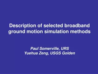
Description of selected broadband ground motion simulation methods Paul Somerville, URS Yuehua Zeng, USGS Golden. Simulation Methods Described: 1. URS 2. Zeng 3. UCSB 4. SDSU. URS Hybrid Approach to Broadband Ground Motion Simulations ( Graves and Pitarka , 2004).

E N D
Description of selected broadband ground motion simulation methods Paul Somerville, URS Yuehua Zeng, USGS Golden
Simulation Methods Described: 1. URS 2. Zeng 3. UCSB 4. SDSU
URS Hybrid Approach to Broadband Ground Motion Simulations • (Graves and Pitarka, 2004)
For f < 1 Hz: • Kinematic representation of heterogeneous rupture on a finite fault • Slip amplitude and rake, rupture time, slip function • 1D FK or 3D FDM approach for Green’s function For f > 1 Hz: • Extension of Boore (1983) with limited kinematic representation of heterogeneous fault rupture • Slip amplitude, rupture time, conic averaged radiation pattern, Stochastic phase • Simplified Green’s functions for 1D velocity structure • Geometrical spreading, impedance effects Both frequency ranges have the nonlinear site amplification based on Vs30 (Campbell and Bozorgnia, 2008)
Kinematic Rupture Generator • Unified scaling rules for rise time, rupture speed and corner frequency • Depth scaling for shallow (< 5 km) moment release: rise time (increase) and rupture speed (decrease) • Scenario Earthquake • Begin with uniform slip having mild taper at edges. • Use Mai and Beroza (2002) spatial correlation functions (Mw dependent, K-2 falloff) with random phasing to specify entire wavenumber spectrum.
Validation Earthquake • Validation events begin with coarse representation from slip inversion. • e.g., Loma Prieta, Wald et al (1991)
Validation Earthquake • Validation events begin with coarse representation from slip inversion. • e.g., Loma Prieta, Wald et al (1991) • Low-pass filter to retain only long wavelength features. Preserves gross asperity locations.
Validation Earthquake • Validation events begin with coarse representation from slip inversion. • e.g., Loma Prieta, Wald et al (1991) • Low-pass filter to retain only long wavelength features. Preserves gross asperity locations. • Extend to fine grid using Mai and Beroza (2002) spatial correlation functions with random phasing for shorter wavelengths.
Rupture Initiation Time Ti = r / Vr – dt(D) Vr = 80% local Vs depth > 8 km = 56% local Vs depth < 5 km linear transition between 5-8 km dt scales with local slip (D) to accelerate or decelerate rupture dt(Davg) = 0
Rise Time t = k · D1/2 depth > 8 km = 2 · k · D1/2 depth < 5 km linear transition between 5-8 km Scales with square root of local slip (D) with constant (k) set so average rise time is given by the Somerville et al (1999, 2009) relations: tA = 1.6e-09 · Mo1/3 (WUS) tA = 3.0e-09 · Mo1/3 (CEUS)
Rake l = lo + e -60o < e < 60o Random perturbations of rake follow spatial distribution given by K-2 falloff.
High Frequency Subfault Source Spectrum • Apply Frankel (1995) convolution operator: • S(f) = C · [ 1 + C · f 2 / fc2 ]-1 • C = Mo / (Nspdl3) N = number of subfaults • sp = stress parameter (50 - WUS), • (125 – CEUS) • dl = subfault dimension • scales to target mainshock moment • scales to mainshock rise time • results generally insensitive to subfault size • Corner frequency scales with local rupture speed (Vr): • fc = co · Vr / (pdl) co = 2.1 (WUS), 1.15 (CEUS) (empirically constrained) • Vr = 80% local Vs depth > 8 km • = 56% local Vs depth < 5 km • linear transition between 5-8 km
Spectral Acceleration Goodness of Fit Ri = ln(Oi /Si) Bias = (1/N) S Ri s = [(1/N) S (Ri – Bias)2]1/2
S-velocity P-velocity
3. UCSB Broadband Strong Motion Synthetics Method Archuleta, Hartzell, Lavallée, Liu, Schmedes Liu, P., R. J. Archuleta and S. H. Hartzell (2006). Prediction of broadband ground-motion time histories: Hybrid low/high-frequency method with correlated random source parameters, Bull. Seismol. Soc. Am. vol. 96, No. 6, pp. 2118-2130, doi: 10.1785/0120060036. Schmedes, J., R. J. Archuleta, and D. Lavallée (2010). Correlation of earthquake source parameters inferred from dynamic rupture simulations, J. Geophys. Res., 115, B03304, doi:10.1029/2009JB006689.
Flowchart for Generating Broadband Strong Motion Synthetics Liu, Archuleta, Hartzell, BSSA
Correlated Source Parameters (LAH) Slip Spatial correlation 30% Average rupture velocity Spatial correlation 60% Rise time (Liu, Archuleta, Hartzell, 2006)
New Kinematic Model (SAL) Schmedes, J., R. J. Archuleta, and D. Lavallée (2010), Correlation of earthquake source parameters inferred from dynamic rupture simulations, J. Geophys. Res., 115, B03304, doi:10.1029/2009JB006689.
High Frequencies Frequency dependent perturbation of strike, dip and rake (Pitarka et al, 2000) ( With f1=1.0 Hz, f2=3.0 Hz Randomness of the high frequencies is generated in the source description.
Ground Motion Computation: 3D • Fourth-order viscoelastic FD code: • Perfectly matched layers • Coarse grained method • Allows for two regions of different grid spacing
Combination of 1D and 3D: Cross correlation at matching frequency fm to align seismograms. Use 3D at frequencies Use 1D at frequencies For
4. Hybrid Broadband Ground-Motion Simulations: Combining Long-Period Deterministic Synthetics with High-Frequency Multiple S-to-S Backscattering Martin Mai, Walter Imperatori, and Kim Olsen Mai, P.M., W. Imperatori, and K.B. Olsen (2010). Hybrid broadband ground-motion simulations: combining long-period deterministic synthetics with high-frequency multiple S-to-S back-scattering, Bull. Seis. Soc. Am. 100, 5A, 2124-2142. Mena, B., P.M. Mai, K.B. Olsen, M.D. Purvance, and J.N. Brune (2010). Hybrid broadband ground motion simulation using scattering Green's functions: application to large magnitude events, Bull. Seis. Soc. Am. 100, 5A, 2143-2162.
Combines low-frequency deterministic synthetics (f ~ 1 Hz) with high-frequency scattering operators • Site effects: • Soil structure • (De-)amplification of ground motions • Non-linear soil behavior • Scattering effects: • inhomogeneities in Earth structure at all scales • scattering model, based on site-kappa, Q, scattering and intrinsicattenuation, hsand hi
Site-Specific Scattering Functions • Scattering Green’s functions computed for each component of motion based on Zeng et al. (1991, 1993) and and P and S arrivals from 3D ray tracing (Hole, 1992) convolved with a dynamically-consistent source-time function, generating 1/f spectral decay • Site-Scattering parameters (scattering and attenuation coefficient, site kappa, intrinsic attenuation) are taken from the literature and are partly based on the site-specific velocity structure. • Assuming scattering operators and moment release originate throughout the fault, but starts at the hypocenter
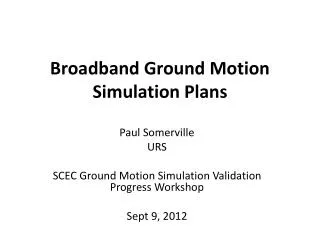
Generation of hybrid broadband seismograms • Hybrid broadband seismograms are calculated from low-frequency and high-frequency synthetics in the frequency domain using a simultaneous amplitude and phase matching algorithm (Mai and Beroza, 2003) Example BB calculation BB 1/f LF SC BB = broadband LF = low frequency SC = scattering functions
Verification and Validation • Method implemented on the SCEC Broadband platform • Validations include Northridge, Landers and Loma Prieta, and NGA relations at selected sites NGA validation at Precariously Balanced Rock sites (Mena et al., 2010) Northridge Validation (Mai et al., 2010)
Comments and issues: • URS and Zeng’s models have considered scaling of rise-time/stress-drop and rupture speed for the upper 5 km depth. • URS, UCSB, Zeng, and SDSU have variable rupture velocities, subevent rakes, rise-time ~ local slip, K-2 fall off in slip distribution • UCSB considered dynamic rupture characteristics for slip time function, correlations between rupture speed, rise time, local slip, … • Matched filter for the hybrid approaches: • - amplitude match • - phase match • - wavelet match 1 Hz
Comments and issues: • URS, UCSB, and SDSU use Green’s functions from 1D/3D wave propagation. Zeng uses 1D Green’s function. They all naturally include body waves and surface waves, Lg and Rg phases for regional wave propagation • Zeng and SDSU use scattering functions for high frequency coda waves • URS, UCSB, Zeng, and SDSU explicitly consider nonlinear soil responses. • URS, UCSB, and SDSU are included in the SCEC computation platform. Zeng is planning to included his.
Input: For all the models: Fault geometry, hypocenter, P- and S-wave velocities, Qp and Qs, fmax, seismic moment, site condition based on Vs30 (nonlinearity), site kappa For URS, UCSB, Olsen, Zeng (except slip): Slip, rise-time, and rupture-time distribution; correlation between these source parameters Variable rake, strike, … In Zeng’s model: slip distribution is defined by subevent stress-drop with random distribution on subevent locations