Lecture 22 Exemplary Inverse Problems including Filter Design
520 likes | 723 Views
Lecture 22 Exemplary Inverse Problems including Filter Design. Syllabus.

Lecture 22 Exemplary Inverse Problems including Filter Design
E N D
Presentation Transcript
Syllabus Lecture 01 Describing Inverse ProblemsLecture 02 Probability and Measurement Error, Part 1Lecture 03 Probability and Measurement Error, Part 2 Lecture 04 The L2 Norm and Simple Least SquaresLecture 05 A Priori Information and Weighted Least SquaredLecture 06 Resolution and Generalized Inverses Lecture 07 Backus-Gilbert Inverse and the Trade Off of Resolution and VarianceLecture 08 The Principle of Maximum LikelihoodLecture 09 Inexact TheoriesLecture 10 Nonuniqueness and Localized AveragesLecture 11 Vector Spaces and Singular Value Decomposition Lecture 12 Equality and Inequality ConstraintsLecture 13 L1 , L∞ Norm Problems and Linear ProgrammingLecture 14 Nonlinear Problems: Grid and Monte Carlo Searches Lecture 15 Nonlinear Problems: Newton’s Method Lecture 16 Nonlinear Problems: Simulated Annealing and Bootstrap Confidence Intervals Lecture 17 Factor AnalysisLecture 18 Varimax Factors, Empircal Orthogonal FunctionsLecture 19 Backus-Gilbert Theory for Continuous Problems; Radon’s ProblemLecture 20 Linear Operators and Their AdjointsLecture 21 Fréchet DerivativesLecture 22 Exemplary Inverse Problems, incl. Filter DesignLecture 23 Exemplary Inverse Problems, incl. Earthquake LocationLecture 24 Exemplary Inverse Problems, incl. Vibrational Problems
Purpose of the Lecture • solve a few exemplary inverse problems • image deblurring • deconvolution filters • minimization of cross-over errors
Part 1 • image deblurring
note that GGT can deduced analytically and is Toeplitz might lead to a computational advantage
Solution Possibilities • Use sparse matrix for G together with mest=G’*((G*G’)\d) (maybe damp a little, too) 2. Use analytic version of GGT together with mest=G’*(GGT\d) (maybe damp a little, too) 3. Use sparse matrix for G together with bicg() to solve GGTλ=d (maybe with a little damping, too) and then use mest=GTλ
Solution Possibilities • Use sparse matrix for G together with mest=G’*((G*G’)\d) (maybe damp a little, too) 2. Use analytic version of GGT together with mest=G’*(GGT\d) (maybe damp a little, too) 3. Use sparse matrix for G together with bicg() to solve GGTλ=d (maybe with a little damping, too) and then use mest=GTλ we used the simplest, which worked fine
image blurred due to camera motion • (100 point blur)
(A) (B) (C) pixel number (D) (E) (F) pixel number pixel number pixel number pixel number
(A) [G-g]728 row number (B) sidelobes R728 pixel number row number
Part 2 • deconvolution filter
Convolution • general relationship for • linear systems • with translational invariance
Convolution • general relationship for • linear systems • with translational invariance model m(t) and data d(t) related by linear operator
Convolution • general relationship for • linear systems • with translational invariance only relative time matters
If the input of a spike m(t)=δ(t) spike causes the output of d(t)=g(t) d(t)= g(t) time , t, after impulse 0 m(t)=δ(t) time , t, after impulse 0
Then the general input m(t) spike of amplitude, m(t0) m(t) time, t t0 causes the general output d(t)=m(t)*g(t) m(t0)g(t-t0) d(t) time, t t0
discrete convolution d=m*g standard matrix from d=Gm
want airgun pulse to be as spiky as possible p(t) = g(t) * r(t) pressure = airgun pulse * sea floor response so as to be able to detect pulses in sea floor response p(t) ≈ r(t)
actual airgun pulse is ringy g(t) time, t
so construct a deconvolutionfilterm(t)so that g(t) *m(t) = δ(t) and apply it to the data p(t) =g(t) * r(t) • p(t)*m(t) = g(t)*m(t)*r(t) = r(t)
so construct a deconvolutionfilterm(t)so that g(t) *m(t) = δ(t) this is the equation we need to solve and apply it to the data p(t) =g(t) r(t) • p(t)*m(t) = g(t)*m(t)*r(t) = r(t)
use discrete approximation of convolution g(t) *m(t) = δ(t) discrete approximation of delta function Gm = d m = ...
solve with damped least squares mest = [GTG + ε2I]-1 GTd • with d = [1, 0, 0, ..., 0]T • (or something similar) • matrices GTG andGTdcan be calculated analytically
approximately Toeplitz with elements autocorrelation of g
Solution Possibilities • Use sparse matrix for G together with mest=(G’*G)\(G’*d) (maybe damping a little, too) 2. Use analytic versions of GTG and GTd together with mest=GTG\GTd (maybe damp a little, too) 3. Never form G, just work with its columns, g use bicg() to solve GTG m = GTd but use conv() to compute GT(Gv) 4. Same as 3 but add a priori information of smoothness
Solution Possibilities • Use sparse matrix for G together with mest=(G’*G)\(G’*d) (maybe damping a little, too) 2. Use analytic versions of GTG and GTd together with mest=GTG\GTd (maybe damp a little, too) 3. Never form G, just work with its columns, g use bicg() to solve GTG m = GTd but use conv() to compute GT(Gv) 4. Same as 3 but add a priori information of smoothness we used this complicated but very fast method
(A) g(t) (B) time, t m(t) (C) time, t m(t)*g(t) time,t
(A) Original d(t) (B) After deconvolution d(t)*m(t)
Part 3 • minimization of cross-over errors
true latitude longitude gravity anomaly, mgal estimated note streaks latitude longitude
general idea data s is measured along tracks data along each track is off by an additive constant theory sjobs (track i) = sjtrue (track i) + m(track i) goal is to estimate the constants by minimizing the error at track intersections
5 cross-over points 6 7 8 4 3 2 1
ith intersection has ascending track Aiand descending track Di sAiobs= sAitrue+ mAi sDiobs= sDitrue+ mDi subtract sAiobs-sDiobs= mAi- mDi has form d=Gm
the matrix G is very sparse every row is all zeros, except for a single +1 and a single-1
note that this problem has an inherent non-uniquenessm is determined only to an overall additive constantone possibility is to use damped least squares, to choose the smallest m(you can always add a constant later)
the matrices GTG and GTd can be calculated semi-analytically
Solution Possibilities • Use sparse matrix for G together with damped least squares mest=(G’*G+e2*speye(M,M))\(G’*d) 2. Use analytic versions of GTG and GTd add damping directly to the diagonal of GTG then use mest=GTGpe2I\GTd 3. Use sparse matrix for G together with bicg() version of damped least squares 4. Methods 1 or 2, but use hard constraint instead of damping to implement Σi mi = 0