Download
1 / 22
220 likes | 240 Views
Explore principled and ad hoc techniques for nuisance parameter handling, hypothesis testing, pivotal quantities, and mixture models at Harvard University. Learn about likelihood ratio tests, posterior predictive assessment, and model checking.

E N D
Dealing with Nuisances: Principled and Ad Hoc Methods Xiao-Li Meng Department of Statistics, Harvard University Joint work with Jingchen Liu (and CHASC) Harvard University
Dealing with Nuisance Parameters • Bringing in a little “Bee”: Posterior Predictive Assessment • Giving up a bit of power: Using an alternative alternative (or a “working” alternative) • Being further away from the big “Bee”: Profiling via moments Harvard University
A Simple Spectral Model • A source spectrum with two components: a continuum modeled by a power law E- , and an emission line modeled as a Gaussian profile with a total flux F. • The expected observed flux Fj from the source within an energy bin Ej for a “perfect” instrument is given by where dEj is the energy width of bin j, and j is the Gaussian proportion in bin j. • If the exact energy is observed, then the distribution follows • Reference: Protassov et al (2002) Harvard University
Hypothesis Testing – Notation • Likelihood L(q|x) = f(x|q), = 0[1, 0\1=; • Null Hypothesis H0: 20 • Alternative Hypothesis HA: 21 • Critical region: C ) Reject null hypothesis if x 2C. • Type I error: P(X 2C | 20) – False negative rate Type II error: P(X 2Cc| 2A) – False positive rate • Power function: p() = P(X 2C | ) • Hypothesis testing of size : p() ·, 8 20 Harvard University
Hypothesis Testing – Likelihood Ratio Test • Uniformly most powerful (UPM) test: the most powerful test among all the tests with size • Likelihood ratio test (LRT): C(c) = {x : LR(x) > c} • In a simple null hypothesis case, if the UMP test exists, it is likelihood ratio test. Harvard University
Seeking Pivotal Quantity • Hypothesis testing of size : max20 P(X 2C | ) = , hard to maximize. • Ideally, we seek a pivotal quantity: T(X) -- its distribution is completely known under the null 0 • Then type I error P(T(X)>t| ) = , 820, • Easy to control type I error, but typically it is very hard to find a useful/powerful pivotal quantity. Harvard University
Posterior Predictive Assessment • p-value = P(T(X) > T(x)| 0), • In the presence of nuisance parameter , under the null, the p-value will be a function of , p() = P(T(X) > T(x) | ). • Posterior predictive p-value: ppp=E(p() | x) = s p() f( | x) d , where f( | x) is the posterior density of . That is, the p-value is calculated under the posterior predictive distribution: f(Xrep|x) = s f(Xrep| 0, ) f( | x) d • Casting doubt on the null hypothesis/model if a ppp is extreme. • Can use realized discrepancy D(X, ): p() = P(D(X , ) > D(x, ) | ). • Can assess the entire posterior distribution of p(). • References: Rubin (1984), Meng (1994), Gelman, Meng and Stern (1996) Harvard University
MODEL 0. There is no emission line. • MODEL 1. There in an emission line with fixed location in the spectrum, but unknown intensity. • MODEL 2. There is an emission line with unknown location and intensity. • Reference: van Dyk & Kang (2004) Harvard University
The posterior predictive check. The two histograms compare the observed likelihood ratio test statistics (vertical lines) with 1000 simulations from the posterior predictive distribution. The left plot is the comparison between Model 0 and Model 1, and the right plot is the comparison between Model 0 and Model 2. Both model checks indicate strong evidence for including the emission line. Harvard University
Mixture Model - Testing p = 0 • Hypothesis testing of mixture model • Particularly, f(x | ) / x-, g(x | , ) = (x| , ) (To avoid singularity at the 0, when > 1, we need to truncate the density away from 0. Without losing generality, we assume x > 1.) • LR is not a pivotal quantity under this model. But if we use a different model for the g component, then we can construct a LR test that is a pivotal quantity. • Let y = log (x) and = 1 / ( - 1), then we can model Harvard University
Difference between the Two Choices Density: normal(1, 0.2) Vs log-normal(0,0.2) Density: normal(1, 0.02) Vs log-normal(0,0.02) Harvard University
Power Comparison: LR under log-normal mixture vs LR under normal mixture when the true model is (almost) normal mixture =1, = 1, = 0.02 are treated as known p = 0.0001, 0.005, 0.01, 0.015, 0.02, 0.03 Only one free parameter, p. =1, = 1, = 0.3 are treated as known p = 0.0001, 0.005, 0.01, 0.015, 0.02, 0.03 Only one free parameter, p. Harvard University
Likelihood Ratio Test and Pivotal Quantity • H0: p = 0, HA: p > 0 • The LRT is pivotal quantity, i.e., the distribution of likelihood ratio is free of . • The maximization can be done via the EM algorithm by viewing the subgroup membership as missing data. Harvard University
Multiple Modes log Likelihood Likelihood of given that = 1, = 0.02, p = 0.01, the sample size is 500 Harvard University
A “Profiled” Likelihood Ratio Test • “Profile likelihood” via moment • Lp( p, , | y) can be maximized via numerical optimization method (the correct likelihood was harder to maximize without using EM). • Let’s define critical region C( c ) = {y | LRp(y) > c} Harvard University
A Sketch of Proof Harvard University
Demonstrating a pivot: QQ-plot of LRs when = 1 vs = 10 Profile Likelihood EM Harvard University
Distribution of 2 log (LR )’s under the null hypothesis Profile Likelihood EM: Starting from E( | y)= 0.5 Harvard University
Power Comparison: “Profile” LRT vs “EM” LRT Harvard University
References • Gelman, A., Meng, X.L., and Stern, H. (1996). Posterior predictive assessment of model fitness via realized discrepancies (with discussions). Statistica Sinica, 6, 733-807 • Meng, X. L. (1994). Posterior predictive p-values. Ann. Stat. 22:1142 - 1160. • Protassov, R., van Dyk, D.A., Connors, A., Kashyap, V.L., and Siemiginowska, A. (2002) Statistics: Handle with Care, Detecting Multiple Model Components with the Likelihood Ratio Test. The Astrophysical Journal, 571:545–559 • Rubin, DB (1984). Bayesianly justifiable and relevant frequency calculations for the applied statistician. Annals of Statistics, 12(4), 1151–1172 • van Dyk, D.A., and Kang, H. (2004). Highly Structured Models for Spectral Analysis in High-Energy Astrophysics. Statistical Science, 9, no. 2, 275–293 Harvard University
Topic “B” reinstated: • How to measure “ego”? • How to classify professions by such “ego” measures? • Finding the most powerful test for testing Ego_Particle Physicists > Ego_Astrophysicists> Ego_Statisticians Harvard University