Download
1 / 82
910 likes | 1.68k Views
CHAPTER (3) : BASIC ELEMENTS OF SUPPLY AND DEMAND. CHAPTER OUTLINE: 1-DEMAND &SUPPLY (D&S) CURVES THE DEMAND CURVE &SHIFTS IN THE (D) CURVE THE SUPPLY CURVE & SHIFTS IN THE (S) CURVE 2-EQUILIBRIUM PRICE (Pe) & QUNTITY (Qe) 3-ADJUSTMENT TO CHANGES IN(D)OR(S),ITS EFFECTS ON (Pe)&(Qe )

E N D
CHAPTER (3) :BASIC ELEMENTS OF SUPPLY AND DEMAND CHAPTER OUTLINE: 1-DEMAND &SUPPLY(D&S) CURVES THE DEMAND CURVE &SHIFTS IN THE (D) CURVE THE SUPPLY CURVE & SHIFTS IN THE (S) CURVE 2-EQUILIBRIUM PRICE (Pe) & QUNTITY (Qe) 3-ADJUSTMENT TO CHANGES IN(D)OR(S),ITS EFFECTS ON(Pe)&(Qe ) 4-GOVERNMENT INTERVENTION IN MARKETS: PRICE CONTROL RENT CONTROL : WHO BENEFITS , WHO LOSES
CHAPTER ( 3 ):DEMAND,SUPPLY & MARKETEQUILIBRIUM I -DEMAND: TOTAL (Qs) THAT CONSUMERS ARE WILLING & ABLE TO BUY AT A CERTAIN (P) AND DURING A PERIOD OF TIME. A- FACTORS AFFECTING(D) FOR (X) COMMODITY: 1- ( Px ) Q Dx THE LAW OF(D):THERE IS AN OPPOSITE RELATIONSHIP B/W (Px) AND (Q Dx) , IF AND ONLY IF WE HOLD OTHER FACTORS CONSTANT. Px 2 4 6 8 10 Qx/DY 500 400 300 200 100 - Px Dx 10 8 6 4 2 Dx Qx 0 100 200 300 400 500
A-DEMAND – FACTORS AFFECTING (Dx) CONT,D + - + 2- INCOME (I): - NORMAL GOODS: ( I ) Dx - INFERIOR GOODS: ( I ) Dx 3- PRICE OF OTHER RELATED GOODS ( Py ): - SUBSTITUTES ( Py ) Dx - COMPLEMENTS ( Py ) Dx 4- TASTE : CONSUMER PREFERANCES WOULD BE AFFECTED BY COMMERCIALS, SEASONALITY, TRADITION ,..etc. 5- NUMBER OF CONSUMERS (# Cs): # Cs Dx 6- CONSUMER EXPECTATIONS(EXP): (P)EXP Dx - + +
CHANGES IN THE DEMAND Px I, Py, T, #Cs, PExp A CHANG IN THE ABOVE FACTOR ONLY WILL CAUSE A MOVEMENT ALONG THE SAME (D) CURVE A CHANGE IN ONE OR ALL OF THE ABOVE FACTORS ONLY WILL CAUSE SHIFTS IN THE (D) CURV Px Px D1 D D + + A D2 10 B 6 D1 D - D D2 Qx Qx 0 0 100 300
Demand & Algebra • Demand - Algebra a- QX = 500 – 2 PX + 0.5 PY + 1.5 I(Demand Function) b- PX = 250 + 0.25 PY+ 0.75 I – 0.5 QX(Inverse Demand Function) - Consumer Surplus • Benefit buyers receive from paying prices less than they’d be willing to pay. • Measured as area below Demand but above Price.
Quiz 2 - Demand__________________________________________________________________________ Name ID# __________________________________________________________________________1. What happens to the demand for SONY color television sets when each of the following happens: a. the price of Mitsubishi TVs rises b. the price of SONY TVs rises c. personal income falls d. dramatic price reductions occur for video recorders e.Government imposes tariffs on Japanese TVs beginning next year2. Suppose the demand for a product (X) can be expressed as a function of its price (Px ), consumer monthly income (I), and the price of a related good Y (PY ) QX = 180 - 10 (Px) - 0.2 (I) + 10 (PY) a. Interpret the slope coefficient on Px b. Is good X a normal or inferior good? Explain. c. Are goods X and Y substitutes or complements? Explain. d. Forgetting income(I) and the price of a related good (Py), how much consumer surplus exists in this market if the price of X were $10?
DEMAND & SUPPLY CURVES CONT”D B-SUPPLY: Qs THAT PRODUCERS ARE WILLING & ABLE TO SELL AT A CERTAIN( P) AND DURING A PERIOD OF TIME. a-FACTORS AFFECTING (S) FOR X COMMODITY: 1-THE (Px) : Q Sx THE LAW OF (S):THERE IS A POSITIVE RELATIONSHIP B/W (Px)AND THE (Q Sx),IF WE HOLD OTHER FACTORS CONSTANT Px 2 4 6 8 10 QSx 100 200 300 400 500 2-PRODUCTION COST (PROD.cost): ( PROD.cost )Sx 3-TECHNOLOGY (TECH): ( BETTER TECH) Sx + Px S 10 8 6 4 - 2 S Qx + 0 100 200 300 400 500
B-SUPPLY CONT’D – FACTORS AFFECTING (Sx) - + 4-FISCAL POLICY:GOV’T POLICIES REGARDING TAXEX & SPENDING HIGHER TAXES LESS Sx (VICE VESA) MORE SUBSIDY MORE Sx (VICE VERSA 5- NUMBER OF PRODUCERS( # PRODx): (# PRDs) Sx 6- PRODUCER’S EXPECTATIONS (P prod exp) : (P prod exp) Sx + -
CHANGES IN THE SUPPLY COST, Py, TECH., #Ps, Pexp, FISCAL POLICY Px A CHANGE IN ONE OR ALL OF THE ABOVE FACTORS ONLY WILL CAUSE SHIFTS IN THE (S) CURV A CHANG IN THE ABOVE FACTOR ONLY WILL CAUSE A MOVEMENT ALONG THE SAME (S) CURVE Px Px s2 S - S S1 A 10 s1 B + 6 S S1 S Qx Qx 0 0 300 500
Supply & Algebra • Supply • Algebra • QX = 500 + 2PX = • Positive relationship between QS and Price • PX = -250 + 0.5QX (Inverse Supply Function) • This is graphed • Producer Surplus • Benefit sellers receive from receiving prices more than they’d be willing to accept • Measured as area above Supply but below Price
EX:THE EQILIBRIUM Pe = 6 AND Qx = 300 Px 2 4 6 8 10 THIS BECAUSE: QDx 500 400 300 200 100 1- Qs = Qd QSx 100 200 300 400 500 2- STABLE , B/C ANY ANY DEVATION FROM THE (Pe) WILL CREATE AUOTOMATIC FORCES ( SHORTAGE OR SURPLUS )THAT WILL BRING THE PRICE BACK TO THE (Pe) 2-DETERMINATION OF THE EQUILIBRIUM (Pe) AND (Qe) Px D S 10 8 Pe 6 4 D 2 S Qx 0 300 100 200 400 500 Qe
3-ADJUSTMENT IN Dx & Sx AND ITS IMPACT ON (Px) &(Qx) A-CHANGES (+&-) IN (Dx) , NO CHANGE IN (Sx ): - INCREASE IN (Dx): - DECREASE IN (Dx) Pe & Qe INCREASE Pe & Qe DECREASE A-CHANGES (+&-) IN (Dx) , NO CHANGE IN (Sx ): - INCREASE IN (Dx): - DECREASE IN (Dx) Pe & Qe INCREASE Pe & Qe DECREASE Sx Sx Px S D2 D2 PX PX D D D 8 8 D1 6 6 6 4 D2 D2 D Sx Sx D D S D1 Qx 0 0 Qx 300 300 400 400 O 200 300
B-CHANGES (+&-) IN (Sx) , NO CHANGE IN (Dx): - INCREASE IN (Sx): - DECREASE IN (Sx ) Pe DECREASE & Qe INCEASE Pe INCREASE & Qe DECREASE PX S2 PX S S S1 D D 8 6 6 S2 4 D S D S S1 Qx Qx 0 0 200 300 400 300
C- CHANGES (+&-) IN BOTH (Sx) &AND (Dx): - INCREASE IN BOTH (Sx)& (Dx): - DECREASE IN BOTH (Sx )&(Dx): Pe INCREASE & Qe INCEASE Pe NO CHANGE & Qe DECREASE B/C + IN Dx > + Sx B/C - IN Dx = - IN Ax PX S2 D1 PX S S S1 D D D2 7 6 6 D1 S2 D S D S D2 S1 Qx Qx 0 0 200 300 300 500
4- GOV’T. INTERVENTION IN MARKETS:A-PRICE CEILING : B- PRICE FLOOR: CAUSE SHORTAGE (AB) CAUSE SURPLUS(CD) Px Px Px Px Px Px Px S D S D D C Pf Pf 8 8 e e 6 6 6 6 6 6 6 A B 4 4 4 4 Pc Pc Pc Pc 4 Pc S D D S Qx Qx 0 0 0 0 400 200 300 200 200 300 300 400 400
CASE STUDY DISCUSSION: RENT CONTROL IN EGYPT Market Pe = 800Ceiling price (P)= 500 Black market (P) = 1000 SHORTAGE = 100,000 UNITS Px S D Black market price 1000 Black market price 1000 Black market price 1000 Black market price 1000 e Marketprice 800 Marketprice 800 Marketprice 800 Marketprice 800 Ceiling price 500 Ceiling price 500 Ceiling price 500 D D S Qx 0 0 0 200,000 200,000 300,000 300,000 100,000 100,000
QUIZ (1)Assume that a Nokia mobile (x) market Pe =1000 and Qe =400 , show this graphically. what will happen if a Samsung mobile market prices increases and the cost of producing the Nokia mobile increased (Make shift in D =shift in S) Px Px Px Px S1 S 1200 1200 1200 1200 1000 1000 1000 1000 D1 D D Ox 0 0 400
Chapter (4) Elasticity • Elasticity • The relative sensitivity of change in one variable (QDx or QSx ) to change in another variable (Px ) • Magnitude of change in the variables • Absolute value of Elasticity greater than, less than or equal to one
Chapter (4) - ELASTICITIES (Cont’d) A- DEMAND ELASTICITIES: • PRICE ELSTICITY OF DEMAND (PED) 1-DEFINITION (PED):THE DEGREE OF RESPONSIVENESS (SESITIVITY) OF THE Q Dx TO THE CHANGES IN THE Px. 2-MEASURING THE(PED): -POINT ELASTICITY FORMULA PEDx = THE SIGN IS NORMALLY( - ) , IF : ∞ >PED > 1 PED=1 0<PED< 1 ELASTIC UNITE ELASTIC INELASTIC EX :LUXTURIES(TRIPS) NECESSITIES(MEDICIN) Q Q x x P P x x
A-DEMAND ELASTICITES:PED (CONT’D) -ARC ELASTICITY FORMULA: PED = THE SIGN NORMALLY( - ) FACTORS DETERMINING PED: 1-TYPE OF THE COMMODITY: BASIC GOODS (BREAD) ARE LESS ELASTIC, WHILE LUXURIES (TRIPS) ARE HIGHLY ELASTIC. 2-NUMBER & DEGREE OF SUBSTITUTES:LESS NUMBER OF SUBSTITUTES(OIL)MEANS LESS PED , WHILE CLOSE SUBSTITUTES (DELL & HP COMPUTER) MEANS HIGH PED. 3-PERCENTAGE OF INCOME SPENT ON THE COMMODITY: IF THE % IS VERY LITTLE (SALT) , THE PED WILL BE LITTLE. 4-THE TIME NEEDED TO ADJUST: IF THE TIME AVAILABLE TO THE CONSUMER IS NOT ENOUGH TO ADJUST TO THE CHANGES IN THE (P) OF A CERTAIN GOOD,THEN THE PED IS LESS AND VICE VERSA . Q1 + Q2 Qx 2 P1 + P2 Px 2
A-DEMAND ELASTICITIES:PED (CONT’D) -THE RELATIONSHIP B/W THE PED & TOTAL REVENUE (TR): 1-PED > 1 ,THEN, THERE IS A NEGATIVE RELATIONSHIP B/W (P) AND (TR). THAT IS WHEN THE (P) , THEN (TR) AND VICE VERSA. 2-PED< 1 , THEN, THERE IS A POSITIVE RELATIONSHIP B/W (P) AND (TR) . THAT IS , WHEN THE (P) , THEN (TR) AND VICE VERSA. 3-PED = 1, THEN, THERE NO CHANGE IN THE(TR) WHEN THE (P) IS CHANGING
A-DEMAND ELASTICITIES: INCOME ELASTICITY OF (D) 2- INCOME ELASTICITY OF DEMAND (IED) IED = THE SIGN COULD BE : ( + ) IF THE GOOD IS NORMAL OR ( - ) IF THE GOOD IS INFERIOR 3- CROSS PRICE ELASTICITY OF DEMAND (CPED): CPED = THE SIGN COULD BE : ( - ) IF GOOD x COMPLEMENT GOOD y ( + ) IF GOOD x SUBSTITUTE GOOD y Qx Qx I I Qx Qx Py Py
B-THE PRICE ELSTICITY OF SUPPLY(PES) PES = THE VALUE COULD TAKE 5 CASES: 1-PES = 0 COMPLETELY INELASTIC 2-PES = ∞ COMPLETELY ELASTIC 3-PES < 1INELASTIC 4-PES = 1 UNIT ELASTIC 5-PES > 1 ELASTIC FACTORS AFFECTING PES 1-FLEXIBILTY IN USING FACTORS OF PRODUCTION 2-TIME NEEDED TO ADJUST PRODUCTION Qsx Qsx Px Px
TRIALTEST 1-WHEN THE SONY TV PRICE DECREASE FROM LE 1000 TO LE 800 , CONSUMERS INCREASED THEIR Q DEMAND FROM 100,000 UNITS/ MONTH TO 120,000 UNITSE /MONTH. CLCULATE THE PED.ALSO , IF THIS IS HAPPENING WHILE THE PRICE OF SAMSUNG TV IS INCRESING FROM LE 500 TO LE 600.THEN CALCULATE THE CROSS-PRICE ELASTICITY.
Equations: Demand ,supply & the Market Equilibrium I- Use the following generalized linear demand relation to answer the following questions: Qx = 680 - 9 Px + 0.006 M – 4 PR 1- where M is income and PR is the price of a related good, R. From this relation it is apparent that the good is: a- an inferior good b- a substitute for good R c- a normal good d- a complement for good R e- both c and d
Equations: Demand ,supply & the Market Equilibrium (Cont’d) • If M = $15,000 and PR = $20, the demand function is Qx = 680 - 9 Px + 0.006 M – 4 PR a. b. c. d. e.
3. If M = $15,000 and PR = $20 and the supply function is , equilibrium price and quantity are, respectively, a. P = $55 and Q = 195. b. P = $9 and Q = 609. c. P = $12 and Q = 200. d. P = $50 and Q = 170. e. P = $40 and Q = 250.
4. If M = $15,000 and PR= $20 and the supply function is , then, when the price of the good is $12 a. there is a shortage of 516 units of the good. B. there is equilibrium in the market. C. there is a surplus of 60 units of the good. D. the quantities demanded and supplied are indeterminate.
5-If M = $15,000 and = $20 and the supply function is , then, when the price of the good is $60, a. there is equilibrium in the market.b. there is a shortage of 180 units of the good.c. there is a surplus of 60 units of the good.d. there is a shortage of 80 units of the good.
II- Use the following demand and supply functions to answer the next 3 questions: Demand: Supply: 1. Equilibrium price and output are a. P = $5 and Q = 30. b. P = $11 and Q = 3.32. c. P = $12 and Q = 44. d. P = $15 and Q = 50. e. none of the above
2.If the price is $10, there is aa. surplus of 30 units. b. shortage of 30 units. c. surplus of 40 units. d. shortage of 10 units. e. none of the above3. If the price is $2, there is a a. surplus of 10 units. b. shortage of 10 units. c. surplus of 30 units. d. shortage of 18 units. e. none of the above
Chapter (5) Demand Estimations 1) The Regression Analysis Elfiky Company uses the per capita income (in thousand LE) to help forecast its demand for computer (brand x) units in million LE . The firm collected the data in the following table (which is presented on annual basis. Year I Dx 2001 5.15 3.25REGRESS : dependent variable (Demand for x 2002 5.05 3.10 computer Using the income per head as 2003 5.25 3.30 independent variable during the period 2004 5.40 3.65 (2000 – 2006) 2005 5.60 3.90 2006 5.70 4.10 • 5.65 4.15
Variable Coefficient Std Err T-statCONST -5.20679 0.616404 -8.44704 (I) 1.63750 0.114037 14.3594No. of Observations = 7 R² = .9763 (adj)= .9716Sum of Sq. Resid. = .260089E-01Std. Error of Reg.= .721234E-01 Durbin-Watson = 2.0012F ( 1, 5) = 206.191 Significance = .05
1-What is the equation of the estimated least squares regression? - Dx = -5.20679 + 1.63750 (I)2-Test the hypothesis that there is no relationship between the dependent and independent variable (at the 95 percent confidence level) in El Fiky Company Regression. Your results indicate that- you would reject the null hypothesis and conclude that the two variables are related
3-The coefficient of determination for this El Fiky Company regression indicates that- 97.63 percent of the variation in Dx is explained by variation in (I)4-Suppose that per capta income 6,300 is expected in 2007. What would be the estimate of El Fiky Company's demand for its coputer in year 2007 ?a. $ 4.62 million b. $ 4.95 million c. $ 4.99 million d. $ 5.11 million
2- An equation is estimated as:QDx = 400 - 2.0 (Px) + 0.015 (I) - 0.17Py (250) (1.0) (0.010) (0.10)standard errors are in parentheses1.The most statistically significant coefficient a. is the constant term.b. The most significant coefficient is of Px .c. The most significant coefficient is of I .d. The most significant coefficient is of Py .
2-The statistic used to test whether the independent variables taken as group statistically explain variation in the dependent variable is the a. R-squared statistic. b. t-statistic. c. Durbin-Watson statistic. d. F-test statistic.3- Serial correlation occurs when a. independent variables are correlated across observations. b. dependent variables are correlated across observations. c. error terms are correlated across observations. d. R-squared is near one and the t-statistics are near zero.
4-The statistic that tests an individual coefficient for statistical significance is the a. R-squared statistic. b. t-statistic. c. Durbin-Watson statistic. d. F-test statistic.5- Multiple regression differs from simple regression in that a. there can be multiple dependent variables. b. the time periods over which observations are taken are multiplied to increase explanatory power. c. a simple regression is done multiple times to increase explanatory power. d. there are multiple independent variables.
Chapter 6:Forecasting • Forecast helps in two areas: 1- Setting cos. Objectives. 2- Constructing cos. business plans. • Subjects of Forecast: 1- Macroecon. Level 2- Sector level 3- Industry level 4- Product level
Demand Estimate & Forecasting • Prerequisite of a good forecast 1- Consistency with other parts of the business. 2- Adequate knowledge of the relevant past. 3- Take into consideration the econ. & political environment. 4- Conducted in timely fashion
Forecasting Techniques Classified into: A- Qualitative Techs: Based on personal judgments 1- Expert Opinion. 2- Opinion Polls & Market research. 3- Surveys of spending plans. B- Quantitative Techs: Utilize significant amount of historical data as a basis for prediction. 1- Naïve 2 - Explanatory 4- Econ. Indicators. 5- Projections. 6- Econometric models.
1- Expert Opinion • Various types of techs: Choosing the most important. 1- The jury of executive opinion. 2- Soliciting the views of the sales staff in a co. to forecast sales. 3- Delphi method.
Opinion Polls & Market research. Dealing with specific products and are often conducted by individual firms. A- Opinion Polls. • Conducted on samples of population. • Choice of the representative sample is of utmost importance. B- Market research. (very close to the opinion polls)
3- Surveys of spending plans. • Quite similar to opinion poll & market research, but it seeks information about macro-type data relating to the economy. • it includes: 1- Consumer intentions. 2- Inventories and sales expectations. 3- Capital expenditure surveys.
B-Quantitative Techs. 4- Econ. Indicators. • Designed to alert business communities to changes in general econ. Conditions. • There are 3 major series of indicators: -Leading, tells us where we are going, where we are, and where we have been. - Coincident, identifies peaks and troughs. - Lagging, confers upturns and downturns in econ. activities.
5- Projections. • A quantitative technique ,naïve metod of forecasting. - past data are projected into the future without taking into consideration reasons for the change, It is simply assumed that the past trends will continue in the future. - Classification: 1- Constant compound growth rate. 2- Visual time series projection. 3- Time series projection using the least squares method
6- Econometrics models. • Causal or explanatory models 1- Single equation model a- Uni-variate : Dx = f(Px) ; Dx = a + b1 Px b- multi-variate ; Dx = a + b1 (Px)+ b2 (Py)+ b3 (I) 2- multi-equation model. Dx = a + bPx ------------------------------------ (1) Sx = c + dPx -------------------------------------- (2) Dx = Sx----------------------------------- (3)
Time series regression model • Single equation-multi-variete model Ex. Demand for automobile: ∆ R = a0 + a1 ∆Y+ a2 ∆P/M + a3 ∆S + a4 ∆X Where: R= retail sales, in millions of new cars. Y= real disposable income. P= real retail price of new cars. M= average credit terms (no. of months of the average installment contract) S= Existing stock, in millions of cars. X= Dummy variable.
Demand for computers Log (yt /yt-1) = a0 + a1 log Pt – a2 log Yt-1 Where Yt = Stock of comps. In yr. t. Yt-1= Stock of comps. In yr. t-1. P = real price of comps.