Download
1 / 45
470 likes | 724 Views
Flow and congestion control. Basic concept of flow and congestion control. Flow control: end-to-end mechanism for regulating traffic between source and destination Congestion control: mechanism used by the network to limit congestion

E N D
Basic concept of flow and congestion control • Flow control: end-to-end mechanism for regulating traffic between source and destination • Congestion control: mechanism used by the network to limit congestion • In either case, both amount to mechanisms for limiting the amount of traffic entering the network • Under circumstances when the load is more than the network can handle
The flow control problem • Consider file transfer • Sender sends a stream of packets representing fragments of a file • Sender should try to match rate at which receiver and network can process data • Can’t send too slow or too fast • Too slow • wastes time • Too fast • can lead to buffer overflow • How to find the correct rate?
Reasons to do flow control • Maximize network throughput • Reduce network delays • Fairness • Tradeoff between fairness, delay, throughput…
One example of flow control • For max through put • Allocate 1 unit for rate a, b and c, 0 for d • For better fairness • Allocate ½ unit to each flow, achieving 2 units of throughput • Or give ¾ unit to a, b and c, ¼ to d, thus each flow consumes same amount of resources, total throughput is 2.5 units d 1 2 3 4 Link capacity: 1 unit a b c
Classification of flow control • Open loop • Source describes its desired flow rate • Network admits call • Source sends at this rate • Closed loop • Source monitors available service rate • Explicit or implicit • Sends at this rate • Due to speed of light delay, errors are bound to occur • Hybrid • Source asks for some minimum rate • But can send more, if available
Open loop flow control • Two phases • Call setup • Data transmission • Call setup • Network prescribes parameters • User chooses parameter values • Network admits or denies call • Data transmission • User sends within parameter range • Network polices users • Scheduling policies give user QoS
Hard problems • Choosing a descriptor at a source • Choosing a scheduling discipline at intermediate network elements • Admitting calls so that their performance objectives are met (call admission control). Daily traffic volume Yearly traffic volume
Traffic descriptors • Usually an envelope • Constrains worst case behavior • Requirements • Representativity: adequately describes flow, so that network does not reserve too little or too much resource • Verifiability: verify that descriptor holds • Preservability: Doesn’t change inside the network • Usability: Easy to describe and use for admission control • Examples • Representative, verifiable, but not usable • Time series of inter-arrival times • Verifiable, preservable, and usable, but not representative • peak rate
Some common descriptors • Peak rate • Average rate • Linear bounded arrival process
Peak rate • Highest ‘rate’ at which a source can send data • Two ways to compute it • For networks with fixed-size packets • min inter-packet spacing • For networks with variable-size packets • highest rate over all intervals of a particular duration • Regulator for fixed-size packets • timer set on packet transmission • if timer expires, send packet, if any • Problem • sensitive to extremes
Average rate • Rate over some time period (window) • Less susceptible to outliers • Parameters: t and a • Two types: jumping window and moving window • Jumping window • over consecutive intervals of length t, only a bits sent • regulator reinitializes every interval • Moving window • over all intervals of length t, only a bits sent • regulator forgets packet sent more than t seconds ago
Linear Bounded Arrival Process • Source bounds # bits sent in any time interval by a linear function of time • the number of bits transmitted in any active interval of length t is less thanrt + W • r is the long term rate • W is the burst limit • Small W strict rate control • Large W allows for larger burst • W = 0 ? • An inactive sender will earn permits so that it can burst later • insensitive to outliers
The leaky bucket rate control Tokens arrive at a rate of r, or one arrival each 1/r seconds • A regulator for a Linear Bounded Arrival Process (LBAP) • Operations of the token bucket • Token enters the bucket at rate r • As long as there are tokens available in the bucket, packets can be sent immediately • If there is no token in the bucket, packets have to wait in the buffer • Largest number of tokens < W • In some cases, r and W can be adjusted to handle congestions
Queueing analysis of leaky bucket • Want to know the performance of the leaky bucket • How long we have to wait to get the token? • A packet may arrive to find • Some packets waiting in queue experience some queueing delay • No packets and token bucket is not empty no queueing delay • Can be formulated into a Markov chain • Slotted time system with a state change each 1/r seconds • A token arrives at the start of the slot and is discarded if bucket is full • Packets arrive according to Poisson process with rate λ • ai = Prob(i arrivals) = (λ/r)ie-(λ/r)/i! Packet arrival 1/r Token arrival
Markov chain formulation of leaky bucket • Let the state of the system • State 0..W-i: W-i token available and no packet waiting, W>=i>=0 • State W+1..W+j: no taken available and j packets waiting in queue, j>0 a4 a3 a2 a2 a2 a1 a2 a1 W+1 W+2 0 1 2 W a0+a1 a0 a0 a0 a0 a0 a0 No packets waiting in queue No token in bucket
The results , and hence pi
Open loop vs. closed loop • Open loop • describe traffic • network admits/reserves resources • regulation/policing • Closed loop • can’t describe traffic or network doesn’t support reservation • monitor available bandwidth • perhaps allocated using GPS-emulation • adapt to it • if not done properly either • too much loss • unnecessary delay
Explicit vs. Implicit • Explicit • Network tells source its current rate • Better control • More overhead • Implicit • Endpoint figures out rate by looking at network • Less overhead • Ideally, want overhead of implicit with effectiveness of explicit
On-off • Receiver gives ON and OFF signals • If ON, send at full speed • If OFF, stop • OK when RTT is small • What if OFF is lost? • Bursty • Used in serial lines or LANs
Flow control window • Recall window based ARQ in data link layer • For error control (retransmissions) • Largest number of packet outstanding (sent but not acked) • If endpoint has sent all packets in window, it must wait, thus slows down its rate • Thus, window provides both error control and flow control • This is called transmission window • Coupling can be a problem • Few buffers are receiver => slow rate!
End to end window DATA • Let • x be expected packet transmission time, • W be size of window, • d be the total round trip delay for a packet • We want flow control only active when there is congestion (want sender to slow down) • Therefore, Wx should be large relative to the total round trip delay d in the absence of congestion • When d < Wx, flow control not active and sending rate is 1/r • When d > Wx, flow control active, and sending rate is smaller than W/d packets per second S D ACK Wx Wx d d W = 6 W = 6 Flow control not active Flow control active
Behavior of end-end windows Actual flow rate = min {1/x, W/d} packets per second • As d increases, flow control becomes active and limits the transmission rate • As congestion is alleviated, d will decrease and r will go back up • Flow control has the affect of stabilizing delays in the network
Choice of window size • Without congestion, window should be large enough to allow transmission at full rate of 1/x packets per second • Let • d’ = the round-trip delay when there is no queueing • N = number of nodes along the path • Dp = the propagation delay along the path • d’ = 2Nx + 2 Dp (delay for sending packet and ack along N links) • Wx > d’ => W > 2N + Dp/x • When Dp < x, W ~ 2N (window size is independent of prop. Delay) • When Dp >> Nx, W ~ 2Dp/x (window size is independent on path length)
Node by node windows • Separate window (w) for each link along the sessions path • Buffer of size w at each node • An ACK is returned on one link when a packet is released to the next link • buffer will never overflow • If one link becomes congested, packets remain in queue and ACKs don't go back on previous link, which would in-turn also become congested and stop sending ACKs (back pressure) • Buffers will fill-up at successive nodes • Under congestion, packets are spread out evenly on path rather than accumulated at congestion point • In high-speed networks this still requires large windows and hence large buffers at each node
TCP Flow Control • Implicit • Dynamic window • End-to-end • Features • no support from routers • Window increase if no loss (usually detected using timeout) • window decrease on a timeout • additive increase and multiplicative decrease
TCP details • Window starts at 1 • Increases exponentially for a while, then linearly • Exponentially => doubles every RTT • Linearly => increases by 1 every RTT • During exponential phase, every ack results in window increase by 1 • During linear phase, window increases by 1 when # acks = window size • Exponential phase is called slow start • Linear phase is called congestion avoidance
More TCP details • On a loss, current window size is stored in a variable called slow start threshold or ssthresh • Switch from exponential to linear (slow start to congestion avoidance) when window size reaches threshold • Loss detected either with timeout or fast retransmit (duplicate cumulative acks) • When a loss is detected: two versions of TCP • Tahoe: in both cases, drop window to 1 • Reno: on timeout, drop window to 1, and on fast retransmit drop window to half previous size (also, increase window on subsequent acks)
Evaluation • Effective over a wide range of bandwidths • A lot of operational experience • Weaknesses • loss => overload? (wireless) • overload => self-blame, problem with FCFS • overload detected only on a loss • in steady state, source induces loss
TCP Vegas • Expected throughput = transmission_window_size/propagation_delay • Numerator: known • Denominator: measure smallest RTT • Also know actual throughput • Difference = how much to reduce/increase rate • Algorithm • send a special packet • on ack, compute expected and actual throughput • (expected - actual)* RTT packets in bottleneck buffer • adjust sending rate if this is too large • Works better than TCP Reno
Congestion control Congestion 3 6 Controlled Throughput 1 4 Uncontrolled 8 2 7 5 Network load Network congestion examples Network throughput when there is (isn’t) congestion control
Networks: Congestion Control Congestion Control • Host-Centric • TCP Congestion Control Mechanisms • Router-Centric • Queuing Algorithms at the router
Networks: Congestion Control Router-Centric Congestion • Queues at outgoing link drop packets to implicitly signal congestion to TCP sources. • Choices in queuing algorithms: • FIFO (FCFS) Drop-Tail • Fair Queuing (FQ) • Weighted Fair Queuing (WFQ) • Random Early Detection (RED) • Explicit Congestion Notification (ECN)
Drop Tail Router • FIFO queueing mechanism that drops packets when the queue overflows. • Introduces global synchronization when packets are dropped from several connections. Networks: Congestion Control
Random Early Detection Implemented on routers When queue length > threshhold 1, start to drop packets randomly When queue length > threshhold 2, drop all incoming packets Can avoid synchronization Can implement differentiated service partly (drop with different weight/threshhold)
TCP congestion control Congestion occurs Congestion 20 avoidance 15 Congestion window Threshold 10 Slow start 5 0 Round-trip times
Comparison among closed-loop schemes • On-off, end to end window, node by node window, TCP and others • Which is best? No simple answer • Some rules of thumb • flow control easier with RR scheduling • otherwise, assume cooperation, or police rates • explicit schemes are more robust • hop-by-hop schemes are more responsive, but more complex • try to separate error control and flow control • rate based schemes are inherently unstable unless well-engineered
Hybrid flow control • Source gets a minimum rate, but can use more • All problems of both open loop and closed loop flow control • Resource partitioning problem • what fraction can be reserved? • how?
Pricing as a way to avoid congestion • Observations • Users are price sensitive • Price can thus be used to influence user’s behavior • Evaluation criteria • Compliance with existing technologies • Measurement requirements for billing and accounting • Support for congestion control or traffic management • Provision of individual QoS guarantees • Degree of network efficiency • Degree of economic efficiency • Impact on social fairness • Pricing time frame
Examples of pricing strategies • Flat pricing • Priority pricing • Paris-Metro pricing • Smart-market pricing • Edge pricing • Expected capacity pricing • Responsive pricing • Effective bandwidth pricing • Proportional fairness pricing - Matthias Falkner, Michael Devetsikiotis, and ioannisLambadaris, An overview of pricing concenpts for broadband IP networks,IEEE Communications Surveys & Tutorials, vol. 3, no. 2, Second Quarter 2000 pp. 2-13 - Luiz A. DaSilva, Pricing for QoS-enabled networks: A survey, IEEE Communications Surveys & Tutorials, vol. 3, no. 2, Second Quarter 2000 pp. 2-8
Flat pricing • Flat charge regardless of usage • Strengths • Simple and convenient • No measurement requirement • Socially fair • Weakness • Unable to reduce/control congestions • No user differentiation • …
Paris-Metro Pricing • Total network bandwidth is divided into several sub-networks (logical) • Each network operates in a best-effort way, but prices differently • Users choose one of logical networks to transmit their traffic (according to their budget) • “higher priced networks can be less congested because users are price sensitive” • Strengths • Simple, like flat pricing • Weakness • Need measurement • Unable to reduce/control congestions within a subnet • No individual QoS • Instability in case of congestion (users may switch between subnets)
PRIORITY PRICING • Can be implemented in a priority-based network • Users are forced to indicate the value of their traffic by selecting a priority level • During periods of congestion the network can then carry the traffic by the indicated level • Strengths • Increases the economic efficiency of the network • Weakness • Measurement needed • Complex to implement • Fairness issues (even you paid, you may be starved because others paid more)
Smart-market pricing • The user associates a price (as bid) with each packet • The network collects and sorts all the bids, and transmit the packets with bids higher than a threshhold • Strengths • Increases network utility (efficiency) • Traffic differentiation • Weakness • Not compatible with existing networks • Difficult to implement • Fairness issue
One recent article from IEEE spectrum • Bob Briscoe, A fair, faster internet, IEEE spectrum, Dec. 2008