A Suitable Bias Correction for CFS Hindcast and Forecast

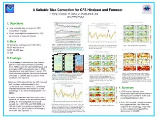
1. A Suitable Bias Correction for CFS Hindcast and Forecast P. Peng, A Kumar, W. Wang, Q. Zhang and B. Jha CPC/NWS/NOAA 1. Objectives a. Have a suitable bias correction for CFS hindcast and forecast; b. Give a more objective assessment for CFS performance in seasonal forecast. 2. Data CFS hindcast for the period of 1981-2004, NCEP Reanalyses-2, NCEP GODAS data, OI SST. Figure 1   Temperature profiles per month used for GODAS in five consecutive latitude bands.  The third panel from the top shows that in the tropics (10S-10N) there was a big increase of observational data from the Expendable Bathythermograph (XBT) and the Tropical Atmosphere Ocean Array of Moored Buoys (TAO) around 1990. Figure 4 Same as Fig. 3 except the forecasted anomalies are adjusted to be with respect to the climatology before and after 1990 respectively Figure 7 Same as Fig.5 except for precipitation. 3. Findings • The increase of observational data used for global oceanic data assimilation (GODAS) since 1990 caused the assimilated tropical and subtropical SST systematically lower (~0.5C) than previous time (see Figures 1 and 2). CFS hindcasts showed similar discontinuity because of the use of GODAS data as oceanic initial conditions (see Figure 3) • Because of the discontinuity, the CFS hindcast skill has been underestimated by the conventional bias correction (i.e., calculating forecasted anomalies with respect to model climatology of the whole hindcast period (1981-2004)). • A more suitable bias correction is proposed to minimize the impact of the discontinuity, that is, dividing the hindcast period into two sub-periods (i.e., 1981-1989 and 1990-2004) and defining model forecasted anomalies as the deviations from the sub-period climatology of the model (see Figures 5-7). Figure 8 The absolute value of the difference between the climatology of the two sub-periods (upper), estimated variability (standard deviation) of the 13-year climatology (middle), and the ratio of the two quantities (lower). The ratio indicates the significance of the difference in climatology between the two sub-periods. The left and right panels are for one month lead and two month lead forecasts respectively. Figure 2   The longitude-time plots of the tropical (10S-10N) SST anomalies.  From the left to the right panels are GODAS SST, Optimum Interpolation (OI) SST and their difference, respectively.  The discontinuity of the GODAS SST bias around 1990 is evident as shown in the right panel. Figure 5 Anomaly correlation (AC) skill of surface air temperature with the whole period based bias correction (upper), sub-period based bias correction (middle) and their difference. The left is for one month lead forecast and the right is for six month lead forecast. 4. Summary • CFS hindcast skill has been significantly improved in many areas of the tropics and subtropics by the sub-period based bias correction. • b. For CFS forecasts, climate anomalies • are suggested to be calculated with respect to the climatology since 1990, so as to mitigate the impact of the discontinuity in GODAS. Figure 3 DJF SST anomaly averaged over the global tropics (10S-10N) for the period of 1982-2004.   The black, red and yellow lines represent the observations (OI SSTs), the ensemble mean of CFS 1-month lead forecasts and the individual members of the CFS forecasts, respectively. It is obvious that in the earlier period (1982-1990), the CFS forecasted SSTs are warmer than the observed, while in the later period the situation is reversed. Figure 6 Same as Fig. 5 except for 200hPa height.