Download
1 / 24
240 likes | 266 Views
Lecture 3. Monte Carlo. Simple Monte Carlo Integration

E N D
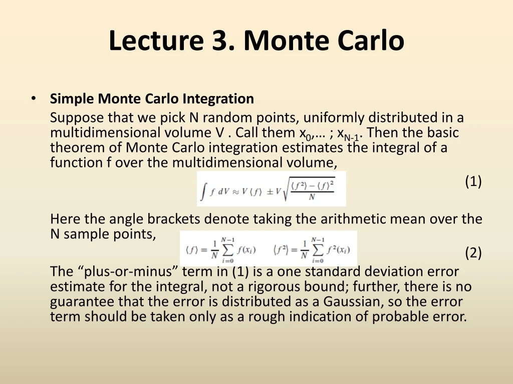
Lecture 3. Monte Carlo • Simple Monte Carlo Integration Suppose that we pick N random points, uniformly distributed in a multidimensional volume V . Call them x0,… ; xN-1. Then the basic theorem of Monte Carlo integration estimates the integral of a function f over the multidimensional volume, (1) Here the angle brackets denote taking the arithmetic mean over the N sample points, (2) The “plus-or-minus” term in (1) is a one standard deviation error estimate for the integral, not a rigorous bound; further, there is no guarantee that the error is distributed as a Gaussian, so the error term should be taken only as a rough indication of probable error.
Suppose that you want to integrate a function g over a region W that is not easy • to sample randomly. For example, W might have a very complicated shape. No • problem. Just find a region V that includes W and that can easily be sampled, and • then define f to be equal to g for points in W and equal to zero for points outside of W (but still inside the sampled V ). You want to try to make V enclose W as closely as possible, because the zero values of f will increase the error estimate term of (1). And well they should: Points chosen outside of W have no information content, so the effective value of N, the number of points, is reduced. The error estimate in (1) takes this into account.
Figure 7.7.1 shows three possible regions V that might be used to sample a • complicated region W . The first, V1, is obviously a poor choice. A good choice, V2, can be sampled by picking a pair of uniform deviates (s; t) and then mapping them • Into (x; y) by a linear transformation. Another good choice, V3, can be sampled by, • first, using a uniform deviate to choose between the left and right rectangular subregions (in proportion to their respective areas!) and, then, using two more deviates to pick a point inside the chosen rectangle. • Let’s create an object that embodies the general scheme described. (We will • discuss the implementing code later.) The general idea is to create an MCintegrate • object by providing (as constructor arguments) the following items: • a vector xlo of lower limits of the coordinates for the rectangular box to be sampled • a vector xhi of upper limits of the coordinates for the rectangular box to be sampled • a vector-valued function funcs that returns as its components one or more • functions that we want to integrate simultaneously • a boolean function that returns whether a point is in the (possibly complicated) • region W that we want to integrate; the point will already be within the region V defined by xlo and xhi • a mapping function to be discussed below, or NULL if there is no mapping • function or if your attention span is too short • a seed for the random number generator
The member function step adds sample points, the number of which is given by its argument. The member function calcanswers updates the vectors ff and fferr, which contain respectively the estimated Monte Carlo integrals of the functions and the errors on these estimates. You can examine these values, and then, if you want, call step and calcanswers again to further reduce the errors.
A worked example will show the underlying simplicity of the method. Suppose that we want to find the weight and the position of the center of mass of an object of complicated shape, namely the intersection of a torus with the faces of a large box. In particular, let the object be defined by the three simultaneous conditions: (torus centered on the origin with major radius D 3, minor radius D 1) (two faces of the box). Suppose for the moment that the object has a constant density ρ = 1.
We want to estimate the following integrals over the interior of the complicated object: The coordinates of the center of mass will be the ratio of the latter three integrals (linear moments) to the first one (the weight). To use the MCintegrate object, we first write functions that describe the integrands and the region of integration W inside the box V . The code to actually do the integration is now quite simple
Change of Variables A change of variable can often be extremely worthwhile in Monte Carlo integration. Suppose, for example, that we want to evaluate the same integrals, but for a piece of torus whose density is a strong function of z, in fact varying according to (6) One way to do this is, in torusfuncs, simply to replace the statement by the statement This will work, but it is not the best way to proceed. Since (6) falls so rapidly to zero as z decreases (down to its lower limit 1), most sampled points contribute almost nothing to the sum of the weight or moments. These points are effectively wasted, almost as badly as those that fall outside of the region W . A change of variable, exactly as in the transformation methods, solves this problem. Let (7) Then ρdz = ds, and the limits -1 < z < 1 become 0.00135 < s < 29.682.
The MCintegrateobject knows that you might want to do this. If it sees an argument xmapthat is not NULL, it will assume that the sampling region defined by xloand xhi is not in physical space, but rather needs to be mapped into physical space before either the functions or the region boundary are calculated. Thus, to effect our change of variable, we don’t need to modify torusfuncs or torusregion, but we do need to modify xlo and xhi, as well as supply the following function for the argument xmap: Code for the actual integration now looks like this: If you think for a minute, you will realize that equation (7) was useful only because the part of the integrand that we wanted to eliminate (e5z) was both integrable analytically and had an integral that could be analytically inverted. In general these properties will not hold. Question: What then? Answer: Pull out of the integrand the “best” factor that can be integrated and inverted. The criterion for “best” is to try to reduce the remaining integrand to a function that is as close as possible to constant.
The limiting case is instructive: If you manage to make the integrand f exactly constant, and if the region V , of known volume, exactly encloses the desired region W , then the average of f that you compute will be exactly its constant value, and the error estimate in equation (1) will exactly vanish. You will, in fact, have done the integral exactly, and the Monte Carlo numerical evaluations are superfluous. So, backing off from the extreme limiting case, to the extent that you are able to make f approximately constant by change of variable, and to the extent that you can sample a region only slightly larger than W , you will increase the accuracy of theMonteCarlo integral. This technique is generically called reduction of variance in the literature. The fundamental disadvantage of simple Monte Carlo integration is that its accuracy increases only as the square root of N, the number of sampled points. If your accuracy requirements are modest, or if your computer is large, then the technique is highly recommended as one of great generality. Later we will see that there are techniques available for “breaking the square root of N barrier” and achieving, at least in some cases, higher accuracy with fewer function evaluations. There should be nothing surprising in the implementation of MCintegrate. The constructor stores pointers to the user functions, makes an otherwise superfluous call to funcsjust to find out the size of returned vector, and then sizes the sum and answer vectors accordingly. The step and calcanswer methods implement exactly equations (1) and (2).
Quasi- (that is, Sub-) Random Sequences We have just seen that choosing N points uniformly randomly in an n-dimensional space leads to an error term in Monte Carlo integration that decreases as In essence, each new point sampled adds linearly to an accumulated sum that will become the function average, and also linearly to an accumulated sum of squares that will become the variance (equation 2). The estimated error comes from the square root of this variance, hence the power N-1/2. Just because this square-root convergence is familiar does not, however, mean that it is inevitable. A simple counterexample is to choose sample points that lie on a Cartesian grid, and to sample each grid point exactly once (in whatever order). The Monte Carlo method thus becomes a deterministic quadrature scheme — albeit a simple one — whose fractional error decreases at least as fast as N-1(even faster if the function goes to zero smoothly at the boundaries of the sampled region or is periodic in the region). The trouble with a grid is that one has to decide in advance how fine it should be. One is then committed to completing all of its sample points. With a grid, it is not convenient to “sample until” some convergence or termination criterion is met. One might ask if there is not some intermediate scheme, some way to pick sample points “at random,” yet spread out in some self-avoiding way, avoiding the chance clustering that occurs with uniformly random points.
A similar question arises for tasks other than Monte Carlo integration. We might want to search an n-dimensional space for a point where some (locally computable) condition holds. Of course, for the task to be computationally meaningful, there had better be continuity, so that the desired condition will hold in some finite n-dimensional neighborhood. We may not know a priori how large that neighborhood is, however. We want to “sample until” the desired point is found, moving smoothly to finer scales with increasing samples. Is there any way to do this that is better than uncorrelated, random samples? The answer to the above question is “yes.” Sequences of n-tuples that fill n space more uniformly than uncorrelated random points are called quasi-random sequences. That term is somewhat of a misnomer, since there is nothing “random” about quasi-random sequences: They are cleverly crafted to be, in fact, subrandom. The sample points in a quasi-random sequence are, in a precise sense, “maximally avoiding” of each other. A conceptually simple example is Halton’ssequence. In one dimension, the j-thnumber Hj in the sequence is obtained by the following steps: (i) Write j as a number in base b, where b is some prime. (For example, j = 17 in base b = 3 is 122.) (ii) Reverse the digits and put a radix point (i.e., a decimal point base b) in front of the sequence. (In the example, we get 0.221 base 3.) The result is Hj. To get a sequence of n-tuples in n-space, you make each component a Haltonsequence with a different prime base b. Typically, the first n primes are used.
It is not hard to see how Halton’s sequence works: Every time the number of digits in j increases by one place, j ’s digit-reversed fraction becomes a factor of b finer-meshed. Thus the process is one of filling in all the points on a sequence of finer and finer Cartesian grids—and in a kind of maximally spread-out order on each grid (since, e.g., the most rapidly changing digit in j controls the most significant digit of the fraction). Other ways of generating quasi-random sequences have been proposed by Faure, Sobol’, Niederreiter, and others. The Sobol’ sequence generates numbers between zero and one directly as binary fractions of length w bits, from a set of w special binary fractions, Vi; I = 1,2, …, w, called direction numbers. In Sobol’s original method, the j-thnumber Xj is generated by XORing (bitwise exclusive or) together the set of Vi ’s satisfying the criterion on i, “the i-thbit of j is nonzero.” As j increments, in other words, different ones of the Vi ’s flash in and out of Xj on different time scales. V1 alternates between being present and absent most quickly, while Vk goes from present to absent (or vice versa) only every 2k-1steps. Figure 7.8.1 plots the first 1024 points generated by a two-dimensional Sobol’ sequence. One sees that successive points do “know” about the gaps left previously, and keep filling them in, hierarchically.
The Latin Hypercube We mention here the unrelated technique of Latin square or Latin hypercube sampling, which is useful when you must sample an N-dimensional space exceedingly sparsely, at M points. For example, you may want to test the crashworthiness of cars as a simultaneous function of four different design parameters, but with a budget of only three expendable cars. (The issue is not whether this is a good plan —it isn’t—but rather how to make the best of the situation!) The idea is to partition each design parameter (dimension) into M segments, so that the whole space is partitioned into MN cells. (You can choose the segments in each dimension to be equal or unequal, according to taste.) With four parameters and three cars, for example, you end up with 3 x 3 x 3 x 3 = 81 cells. Next, choose M cells to contain the sample points by the following algorithm: Randomly choose one of the MN cells for the first point. Now eliminate all cells that agree with this point on any of its parameters (that is, cross out all cells in the same row, column, etc.), leaving (M – 1)Ncandidates. Randomly choose one of these, eliminate new rows and columns, and continue the process until there is only one cell left, which then contains the final sample point. The result of this construction is that each design parameter will have been tested in every one of its subranges. If the response of the system under test is dominated by one of the design parameters (the main effect), that parameter will be found with this sampling technique. On the other hand, if there are important interaction effects among different design parameters, then the Latin hypercube gives no particular advantage. Use with care. There is a large field in statistics that deals with design of experiments.
Adaptive and Recursive Monte Carlo Methods This section discusses more advanced techniques of Monte Carlo integration. As examples of the use of these techniques, we include two rather different, fairly sophisticated, multidimensional Monte Carlo codes: vegasand miser. The techniques that we discuss all fall under the general rubric of reduction of variance, but are otherwise quite distinct. Importance Sampling The use of importance sampling was already implicit in equations (6) and(7). Suppose that an integrand f can be written as the product of a function h that is almost constant times another, positive, function g. Then its integral over a multidimensional volume V is (11) In equation (7) we interpreted equation (11) as suggesting a change of variable to G, the indefinite integral of g. That made g dVa perfect differential. We then proceeded to use the basic theorem of Monte Carlo integration, equation (1). A more general interpretation of equation (11) is that we can integrate f by instead sampling h — not, however, with uniform probability density dV , but rather with nonuniform density g dV. In this second interpretation, the first interpretation follows as the special case, where the means of generating the nonuniform sampling of g dVis via the transformation method, using the indefinite integral G.
More directly, one can go back and generalize the basic theorem (1) to the case of nonuniform sampling: Suppose that points xi are chosen within the volume V with a probability density p satisfying (12) The generalized fundamental theorem is that the integral of any function f is estimated, using N sample points x0, … , xN-1, by (13) where angle brackets denote arithmetic means over the N points, exactly as in equation (2). As in equation (1), the “plus-or-minus” term is a one standard deviation error estimate. Notice that equation (1) is in fact the special case of equation (13), with p = constant = 1/V . What is the best choice for the sampling density p? Intuitively, we have already seen that the idea is to make h = f/p as close to constant as possible. We can be more rigorous by focusing on the numerator inside the square root in equation (13), which is the variance per sample point. Both angle brackets are themselves Monte Carlo estimators of integrals, so we can write (14)
We now find the optimal p subject to the constraint equation (12) by the functional variation (15) with λa Lagrange multiplier. Note that the middle term does not depend on p. The variation (which comes inside the integrals) gives 0 = -f2 / p2 + λ or (16) where λhas been chosen to enforce the constraint (12). If f has one sign in the region of integration, then we get the obvious result that the optimal choice of p — if one can figure out a practical way of effecting the sampling — is that it be proportional to |f|. Then the variance is reduced to zero. Not so obvious, but seen to be true, is the fact that p ~ |f| is optimal even if f takes on both signs. In that case the variance per sample point (from equations 14 and 16) is (17)
One curiosity is that one can add a constant to the integrand to make it all of one sign, since this changes the integral by a known amount, constant V . Then, the optimal choice of p always gives zero variance, that is, a perfectly accurate integral! The resolution of this seeming paradox is that perfect knowledge of p in equation (16) requires perfect knowledge of ∫|f|dV, which is tantamount to already knowing the integral you are trying to compute! If your function f takes on a known constant value in most of the volume V , it is certainly a good idea to add a constant so as to make that value zero. Having done that, the accuracy attainable by importance sampling depends in practice not on how small equation (17) is, but rather on how small is equation (14) for an implementable p, likely only a crude approximation to the ideal. Stratified Sampling The idea of stratified sampling is quite different from importance sampling. Let us expand our notation slightly and let <<f>> denote the true average of the function f over the volume V (namely the integral divided by V ), while <f> denotes as before the simplest (uniformly sampled) Monte Carlo estimator of that average: (18)
The variance of the estimator, Var(<f>), which measures the square of the error of the Monte Carlo integration, is asymptotically related to the variance of the function, Var (f) = <<f2>> - <<f>>2, by the relation (19) Suppose we divide the volume V into two equal, disjoint subvolumes, denoted a and b, and sample N/2 points in each subvolume. Then another estimator for <<f>>, different from equation (18), which we denote <f>’, is (20) in other words, the mean of the sample averages in the two half-regions. The variance of estimator (20) is given by (21) From the definitions already given, it is not difficult to prove the relation (22)
We have not yet exploited the possibility of sampling the two subvolumes with different numbers of points, say Na in subregion a and Nb= N - Na in subregion b. Let us do so now. Then the variance of the estimator is (23) which is minimized (one can easily verify) when (24) If Na satisfies equation (24), then equation (23) reduces to (25) Equation (25) reduces to equation (19) if Var(f) = Vara (f) = Varb(f), in which case stratifying the sample makes no difference. A standard way to generalize the above result is to consider the volume V divided into more than two equal subregions. One can readily obtain the result that the optimal allocation of sample points among the regions is to have the number of points in each region j proportional to j (that is, the square root of the variance of the function f in that subregion). In spaces of high dimensionality (say d >= 4) this is not in practice very useful, however. Dividing a volume into K segments along each dimension implies Kdsubvolumes, typically much too large a number when one contemplates estimating all the corresponding j ’s.
Adaptive Monte Carlo: VEGAS The VEGAS algorithmiswidely used for multidimensional integrals that occur in elementary particle physics. VEGAS is primarily based on importance sampling, but it also does some stratified sampling if the dimension d is small enough to avoid Kd explosion (specifically, if (K/2)d< N/2, with N the number of sample points). The basic technique for importance sampling in VEGAS is to construct, adaptively, a multidimensional weight function g that is separable, (26) Such a function avoids the Kdexplosion in two ways: (i) It can be stored in the computer as d separate one-dimensional functions, each defined by K tabulated values, say — so that K x d replaces Kd . (ii) It can be sampled as a probability density by consecutively sampling the d one-dimensional functions to obtain coordinate vector components (x; y; z; …). The optimal separable weight function can be shown to be (27)
When the integrand f is concentrated in one, or at most a few, regions in d-space, then the weight function g’s quickly become large at coordinate values that are the projections of these regions onto the coordinate axes. The accuracy of the Monte Carlo integration is then enormously enhanced over what simple Monte Carlo would give. The weakness of VEGAS is the obvious one: To the extent that the projection of the function f onto individual coordinate directions is uniform, VEGAS gives no concentration of sample points in those dimensions. The worst case for VEGAS, e.g., is an integrand that is concentrated close to a body diagonal line, e.g., one from (0;0;0; …) to (1; 1; 1; …). Since this geometry is completely nonseparable, VEGAS can give no advantage at all. More generally, VEGAS may not do well when the integrand is concentrated in one-dimensional (or higher) curved trajectories (or hypersurfaces), unless these happen to be oriented close to the coordinate directions.