Image Filtering and Image Arithmetic
Image Filtering and Image Arithmetic. a. Image Filtering. filters emphasise or de-emphasise image data of various Spatial frequencies spatial frequency refers to roughness of tonal variations in image

Image Filtering and Image Arithmetic
E N D
Presentation Transcript
a. Image Filtering • filters emphasise or de-emphasise image data of various Spatial frequencies • spatial frequency refers to roughness of tonal variations in image • areas of high spatial frequency are tonally rough - grey levels change abruptly over small distances eg. across roads, field borders • smooth areas have low spatial frequency eg. large fields or water bodies
Image filtering • low pass filters emphasise low frequency changes in brightness and de-emphasise local detail eg. smoothing filter (mean, median or mode); noise removal filter • high pass filters emphasise high frequency components of image and de-emphasise more general, low frequency detail eg. edge enhancement filter; directional first differencing filter • pixels modified on basis of grey level of neighbouring pixels in 3 stages:- • input image • moving window (kernel) • output image
Kernel • the kernel is a square matrix (window) which is moved pixel-by-pixel over the image • has an odd numbered array of elements (3x3, 5x5 etc.) whose elements represent a weight to be applied to each corresponding digital number of the input image: result is summarised for central pixel eg. mean
Low pass 3*3 Mean filter other frequencies may be smoothed by altering size of kernel or weighting factors
Traverse of pixel values across raw image and after mean filter
Output image for mean filter • The output value for the central image pixel covered by the kernel(k) is the value of the products of each of the surrounding input pixel values and their corresponding kernel weights (W): O(x,y) = SUMk(x,y/W) /nk Where O = output value for central pixel
Ikonos Pan image of Shau Kei Wan, with raw image, 3*3, 5*5 and 7*7 kernel smoothing filter
Ikonos Pan. image of Mt. Butler/Mt. Parker Before and after 5 * 5 low pass (smoothing) filter
Median smoothing filters • superior to mean filter, as median is an actual number in the dataset (kernel) • less sensitive to error or extreme values • eg. 3,1,2,8,5,3,9,4,27 median=5, mean=6.89 rounded to 7 • 7 not present in original dataset • mean larger than 6 of the 9 observed values because influenced by extreme value 27 (3 times higher than next highest value in dataset) • therefore isolated pixels, which may represent noise removed by median • preserves edges better than mean, which blurs edges (fig.7.2)
Effect of median filtering in noise removal Figure1. SPOT Image before removal of the pushbroom scanner noise. The darker and lighter areas represent differing levels of suspended sediment east of Lamma Island Figure 2. Image after removal of scan (system) noise using a 11*11 median filter. Edges of sediment plumes also preserved
Modal smoothing filter • often referred to as a ‘majority’ filter • used for classified data, as mean and median are irrelevant for class data • removes misclassified ‘salt and pepper’ pixels
High pass (sharpening) filters • emphasise high frequency component by exaggerating local contrast eg. mean of surrounding pixels = 30, central pixel = 30, filtered (180/6) = 30 mean of surrounding pixels = 30, central pixel = 35, filtered (250/6) = 42
Before and after 3 * 3 high pass (sharpening) filter Ikonos Panchromatic, Mt. Butler
Edge Enhancement and Sharpening filters • edges: ‘areas where slope of grey level values change markedly’ • to detect edges, need both high and low frequency information • high pass sharpening filters enhance local contrast but do not preserve low frequency brightness information • edge filters attempt to preserve both • done by first isolating the low frequency component by low pass filtering, then subtract this from original image leaving the high frequency component • add this back to original, doubling the high frequency part after edge filter
Directional First Differencing • part of edge enhancement used for emphasising lineaments in one of four directions • determines the derivative of grey levels with respect to a given direction • compares each pixel to one of its neighbours • result can be positive or negative outside the byte range, so rescaled by adding 127 • first differences often give very small values so contrast stretch is also done
LANDSAT band 2 (green): west of Guangzhou, with Y-directional filter emphasising E-W trends
Noise removal • noise - ‘the unwanted disturbance in an image that is due to limitations in the sensing, digitisation or data recording process’ • may either be systematic (banding of multispectral images) or random eg. dropped lines- these may degrade, or totally mask the true radiometric information content of the digital image • removal is done to produce an image that is as close to the original radiometry of the scene as possible • removal is critical to the subsequent processing and classification of an image
Stripe noise Sixteenth line banding noise in LANDSAT Band 2 (green) of 3.3.96: Deep Bay, Hong Kong
Line drop • Dropped line removed by averaging pixels each side of the line using a 1-dimensional 3*1 vertical filter with threshold of 0
b. Image Arithmetic: band ratioing • enhance image by dividing one band with another • independent of variations in scene illumination • may highlight subtle spectral differences because portray variations in slopes of the spectral curves between two bands, which are different for different materials eg. vegetation is darker in the visible, but brighter in the NIR than soil, thus the ratio difference is greater than either band individually
Ratio images • ratios commonly used as vegetation indices aimed at identifying greenness and biomass • a ratio of NIR/Red is most common • the number of ratios possible from n bands • = n(n-1), thus for SPOT = 6, LANDSAT TM =30 • can be used to generate false colour composites by combining 3 monochromatic ratios
Use of ratio to reduce topographic effects NB. The objective is to map 2 classes –coniferous and deciduous forest
Effects of NIR/RED ratio on topograpic shading SPOT Band 3 (NIR) SPOT Bands 3/ 2 (NIR/Red) Q. Why do we want to reduce topographic shading?
LANDSAT FCC of semi-arid zone, northern Nigeria in dry season, showing effects of displaying Vegetation Index (NDVI) on red NB. in dry season the only green vegetated areas, for growing of crops and cattle grazing are along river valleys and on irrigation schemes
Factors to consider in band ratios • choice of bands important - some bands highly correlated should not be ratioed • only cancels those factors that are operative equally in both bands eg. topographic effects BUT others such as atmospheric factors may be additive • ratioing may enhance noise patterns that are uncorrelated in individual bands • ratio between raw DNs may be different from between radiance values, as offsets different • generally require re-scaling to byte scale
c. Change detection • involves use of multitemporal images to discriminate land cover change between dates • can be short term change eg. flooding or vegetation ripening, or long term eg.urban growth or desertification or sea level change • imagery should be comparable eg. same sensor, bands, spatial resolution, time of day • anniversary dates minimise seasonal and sun angle differences • accurate spatial registration of images important eg. 1/4 to 1/2 pixel
Lillesand and Keifer Plate 9. LANDSAT MSS, Las Vegas Change detection process 1972 1986 • two approaches - • postclassification comparison • temporal image differencing 1992
URBAN WATER SOIL GRASS FOREST TOTAL %Change URBAN 82 6 7 2 3 100 WATER 2 30 0 0 0 32 SOIL 4 4 20 1 0 29 GRASS 4 0 3 18 8 33 FOREST 8 2 3 3 26 42 TOTAL 102 42 33 24 37 236 Post-classification comparison • co-register 2 dates of images and independently classify them • devise algorithm to determine change • eg. IF i1 = i2 THEN null ELSE C • OR • IF i1=1 AND i2=2 THEN C1.2 • IF i1=1 AND i2=3 THEN C1.3 • devise contingency • table
Temporal image differencing (single band) • co-register images of different dates • do atmospheric correction • convert to radiance • subtract image pixel values change image • no change - change image values near zero • areas of change give larger negative or positive values • possible values -255 to +255: rescale by +-, /2, +127 • determine threshold for change • change will be within tails of histogram distribution
SPOT FCC image of Tai Mo Shan, Dec, 1991 showing burn cloud SPOT NIR band
SPOT February 1995 NIR band
Increase in NIR reflectance over burned area from Dec 1991 to Feb.1995
Vegetation change detection based on NIR radiance T1=20, T2=90T1-T2=-70(-70/2)+127=92 Graph of lookup table for mapping change values (0-100, and 150-255) to white Areas of less or no change (101-149) set to black Change Histogram No difference =127 Thresholds for change = <100 and >150