Nonparametric Statistics
STAT E-150 Statistical Methods. Nonparametric Statistics.

Nonparametric Statistics
E N D
Presentation Transcript
STAT E-150Statistical Methods Nonparametric Statistics
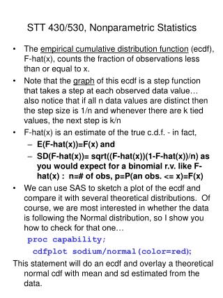
The tests we have discussed generally require that the data meet particular conditions. Nonparametric tests make fewer assumptions about the data; they generally do not require that the data follow any particular distribution, although they often require that the population(s) have continuous distributions. In addition, many nonparametric tests are not based on the actual values of the data. They may use counts of values, or the rank of each observation.
Here is an example: A neurologist may collect data to investigate the depressant effects of certain recreational drugs. She tested 20 clubbers; 10 were given an ecstasy tablet to take on a Saturday night and 10 were allowed to drink only alcohol. Levels of depression were measured using the Beck Depression Inventory (BDI) the day after and at midweek.
The Wilcoxon Rank Sum Test Suppose there is no difference in the depression levels between ecstasy and alcohol users. Rank the data without regard to the group the subject belonged to, giving the lowest value a rank of 1, the next lowest the rank of 2, etc. If there is no difference between the groups we should find similar number of low and high ranks in each group. If we added up the ranks, the sums for each group should be about the same.
What if there is a difference? Suppose the ecstasy group is more depressed than the alcohol group. Then there would be higher ranks in the ecstasy group than in the alcohol group, and the sum of the ranks for the ecstasy group would be higher than the sum for the alcohol group. When the groups are not the same size, the test statistic for the Wilcoxon Rank Sum Test, W, is the sum of the ranks for the smaller group. If the groups are the same size, the test statistic W is the value of the smaller summed rank.
Here are the steps: 1. Draw a simple random sample of size n1 from one population and draw an independent SRS of size n2 from a second population. Rank all N observations. The sum W of the ranks for the first sample is the Wilcoxon rank sum statistic.
If the two populations have the same continuous distribution, then and The Wilcoxon Rank Sum Test rejects the hypothesis that the two populations have identical distributions when the rank sum W is far from its mean. That is, we can use the test statistic
How to rank the data? For the Wednesday data, arrange the values in ascending order, noting the group the subject belonged to. Then start at the lowest score, assigning a rank of 1, and continue ranking all values. When a value occurs more than once, average the ranks.
Sum of ranks for alcohol = Sum of ranks for ecstasy =
The value of the test statistic for Wednesday is If this value is large (>1.96), then the test is significant at α = .05. What can you conclude?
Here are the results for the Sunday data: Sum of ranks for alcohol = Sum of ranks for ecstasy =
Here are the SPSS results: The results for Sunday do not show a significant difference between the two groups (p = .28), but the results for Wednesday indicate that there is a difference in the depression scores for the two groups (p = 0+),
The results for Sunday do not show a significant difference between the two groups (p = .28), but the results for Wednesday indicate that there is a difference in the depression scores for the two groups (p = 0+), That is, this data indicates that ecstasy is no more of a depressant than alcohol one day after taking it, than is alcohol. But for the midweek measures, the difference is significant (p is close to 0). This indicates that the ecstasy group had significantly higher levels of depression midweek than did the alcohol group. Note also that the mean rank for Wednesday scores is higher for the ecstasy users (15.10) than for the alcohol users (5.90).
Using SPSS First create a new coding variable for the nominal data: > Transform > Recode into different variables The input variable is Drug; create a new variable, DrugCode
Code Ecstasy as "1" and click on Add Code Alcohol as "2" and click on Add
Then click on Continue and then click on Change and OK You should see the new column in Data View.
Click on Analyze > Nonparametric Tests > Legacy Dialogs > 2 Independent SamplesChoose BDISunday and BDIWednesday as the Test Variables Choose DrugCode as the Grouping variable Select Mann-Whitney U as the Test Type and click on OK.
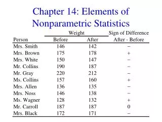
Outliers and Influential Points In linear regression, an outlier is an observation that lies outside the overall pattern for the data. Points that are outliers in the y-direction have large residuals, but other outliers may not. An observation is influential if removing it would remarkably change the overall pattern. Points that are outliers in the x-direction are often influential. Influential points draw the regression line toward themselves, and so they cannot be identified by looking for large residuals. It should be noted that not all outliers are influential.
Child 18 Child 18 Does the age at which a child begins to talk predict a later score on a test of mental ability? This data shows the age in months at which each child spoke his/her first word, and each child’s Gesell Adaptive Score, the result of an ability test taken much later.
The graph of the data shows a negative linear relationship. Child 18 is close to the line but is an outlier in the x-direction. Because of its extreme position on the x-scale, this point has a strong influence on the regression line. It is an influential point. Child 19 is an outlier in the y-direction; the point lies far from the regression line and has a large residual.
Here are the results with all points: without Child 18: without Child 19: What differences do you see when Child 18 is removed? What differences do you see when Child 19 is removed? Which point is influential?