Download
1 / 1
10 likes | 118 Views
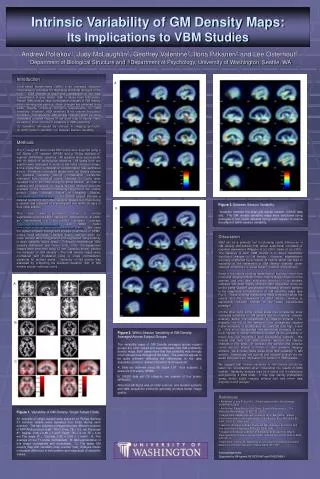
1 Department of Biological Structure and 2 Department of Psychology, University of Washington, Seattle, WA. Introduction

E N D
1Department of Biological Structure and 2Department of Psychology, University of Washington, Seattle, WA Introduction Voxel-based morphometry (VBM) is an unbiased, objective neuroimaging technique for identifying structural changes in the brain. VBM involves a voxel-wise comparison of the local concentration of gray matter (GM) in whole brain MRI scans. Recent VBM studies have investigated changes in GM density due to learning and practice. Such changes are expected to be small, thereby imposing stringent requirements on VBM sensitivity. However, VBM sensitivity is not uniform throughout the brain. Consequently, GM density changes might be more observable in some regions of the brain than in others. Here, we explore three sources of variability in VBM sensitivity: (1) variability introduced by choices in imaging protocols; (2) within session variability; (3) between session variability. A Intrinsic Variability of GM Density Maps: Its Implications to VBM Studies Methods The T1 weighted whole head MRI scans were acquired using a GE Sigma 1.5T scanner (SPGR) and a Philips Achieva 3T scanner (MPRAGE) scanners. All subjects were young adults with no history of neurological disorders. All scans from one session were averaged to obtain a low-noise structural image, and a single ‘best’ normalization transformation was estimated from it. Therefore, normalized results were not directly affected by possible variability among normalization transforms estimated from individual scans. Identical T1 scans were repeated four to six times during the same session. In order to compare and generalize our results, we also analyzed data sets available to the scientific community as part of the OASIS project (Open Access Series of Imaging Studies, http://www.oasis-brains.org/). The OASIS project includes a data set containing 20 normal subjects imaged four times during a session and repeated on a subsequent visit within 90 days of their initial session. The data were processed using a unified segmentation/normalization framework (Ashburner et. al 2005) as implemented in the SPM5 software package (http://www.fil.ion.ucl.ac.uk/spm/) and VBM5 toolkit (http://dbm.neuro.uni-jena.de/vbm/vbm5-for-spm5/). We used the default software settings and analysis parameters of SPM5, unless noted otherwise. Multiple scans obtained within the same session were coregistered and segmented independently in each subject’s native space. Following conventional VBM analysis (Ashburner and Friston, 2000, 2005), the segmented images were smoothed using 12 mm Gaussian kernel, yielding the measure of GM density. The GM density maps were normalized and modulated using a single normalization transform for multiple scans.. Variability of GM density was assessed by computing the standard deviation (SD) of GM density across individual scans Figure 3. Between Session Variability Variability between the scan and rescan session (OASIS data set). The GM density variability maps were calculated using averages of four scans obtained during each session to reduce the effect of within session variability. B Discussion VBM can be a powerful tool for studying subtle differences in GM density distributions that reflect anatomical correlates of cognitive parameters (Maguire et al., 2000, Gaser et al., 2003). The objective of such VBM studies is to detect statistically significant changes in GM density. However, segmentation accuracy is affected by a number of factors which can lead to variability in the estimation of GM density obtained under identical conditions (i.e. same subject, scanner and protocol). Some of the factors affecting segmentation accuracy result from noise and imaging artifacts; these factors largely depend on the scanner and the data acquisition protocol. Our analysis indicates that even slightly different data acquisition protocols on the same scanner can produce noticeably different patterns in the magnitude and distribution of GM variability maps (see Fig.1). These differing distributions could potentially affect the results and the conclusions of VBM studies, leading to significantly different findings for the same experimental paradigm. On the other hand, some cortical areas may consistently show increased variability in GM density due to relatively complex anatomy and/or the persistence of imaging artifacts. For example, the tip of the temporal lobe consistently showed higher variability in all data sets we analyzed (see Figs. 2 and 3). This is not unexpected considering the proximity of non-brain tissues of similar intensities, as well as the possibility of blood flow, eye movement and susceptibility artifacts. We noticed that very few VBM studies reported GM density changes it this area. In contrast, the parietal and occipital cortex are not subject to these or other common imaging artifacts. As a result, these areas show little variability in GM density. Interestingly, the parietal and occipital cortices are the areas that have been implicated in a number of VBM studies. We suggest that intrinsic variability of GM density should be taken into consideration when interpreting the results of VBM studies. Variability analysis may be a useful tool for designing and planning a VBM study. It may help identify problematic areas, detect subtle imaging artifacts and help refine data acquisition and analysis. Andrew Poliakov1, Judy McLaughlin2, Geoffrey Valentine2, Ilona Pitkanen2 and Lee Osterhout2 A B Figure 2. Within Session Variability of GM Density: Averaged Across Subject Groups The variability maps of GM Density averaged across subject groups are color coded and superimposed onto GM probability density maps. Both cases show that that variability was strongly non-homogenious throughout the brain. The patterns appear to be quite different reflecting the differences in the data acquisition protocol, artifact correction techniques etc. A. Data set obtained using GE Signa 1.5T (four subjects, 2 sessions of 6 scans, SPGR). B. OASIS data set (15 subjects, two session of four scans, MPRAGE). Note that GE Signa was an older scanner, and modern systems and data acquisition protocols generally produce better image quality. C • References • Ashburner J. and Friston K.J. Unified segmentation. NeuroImage, 26:839-851, 2005. • Ashburner J. and Friston. K.J. Voxel-Based Morphometry -- The Methods. NeuroImage, 11:805-821, 2000. • Maguire EA, Gadian DG, Johnsrude IS, et al. Navigation-related structural change in the hippocampi of taxi drivers. Proc Natl Acad Sci USA. 2000; 97: 4398-4403. • Gaser C, Schlaug G. Brain structures differ between musicians and non-musicians. J Neurosci 2003; 23: 9240-9245. • Draganski B, Gaser C, Busch V, Schuierer G, Bogdahn U, May A. Neuroplasticity: changes in grey matter induced by training. Nature 2004; 427: 311-2. • Mechelli A, Crinion JT, Noppeney U, et al. Neurolinguistics: structural plasticity in the bilingual brain. Nature 2004; 431: 757. • Acknowledgements • Supported by NIH grants R01DC01947 and P30DC04661 Figure 1. Variability of GM Density: Single Subject Data An example of single subject data acquired on Philips Achieva 3T scanner (scans were repeated four times during each session). The two columns correspond to two different versions of MPRAGE protocol (Left : TR=7.5 ms, TE = 3.5, ms Flip angle 80 ; Sagital, 0.86 x 0.86 x 1 mm3; Right: TR=7.4 ms TE = 3.44 ms Flip angle 80 ; Coronal, 0.92 x 0.92 x 1 mm3). A. The average of four T1 scans (normalized). B. GM segmentation of this image (normalized and modulated). C. The mean GM density map with variability map overlaid (red). Analysis shows noticeable difference in both pattern and magnitude of variability values.