Chapter 5 – Density estimation based on distances

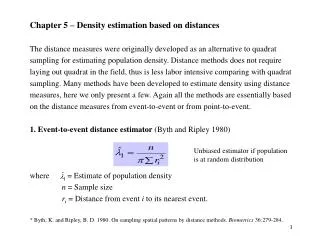
1. Chapter 5 – Density estimation based on distances • The distance measures were originally developed as an alternative to quadrat sampling for estimating population density. Distance methods does not require laying out quadrat in the field, thus is less labor intensive comparing with quadrat sampling. Many methods have been developed to estimate density using distance measures, here we only present a few. Again all the methods are essentially based on the distance measures from event-to-event or from point-to-event. • 1. Event-to-event distance estimator (Byth and Ripley 1980) • where = Estimate of population density • n = Sample size • ri = Distance from event i to its nearest event. • * Byth, K. and Ripley, B. D. 1980. On sampling spatial patterns by distance methods. Biometrics 36:279-284. Unbiased estimator if population is at random distribution

2. 2. Point-to-event distance estimator (Byth and Ripley 1980) • where = Estimate of population density • n = Sample size • xi = Distance from random point i to its nearest event. • It is obvious that estimators 1 and 2 are of the same mathematical form. They also share the same variance which can be used to construct confidence intervals for the estimates. The variance is given for the inverse of the density as follows. • Note: The CI for  is obtained by the inverse of the CI for 1/. Unbiased estimator if population is at random distribution

3. 3. Geometric mean estimator of N1 and N2(Diggle 1975) • where = Event-to-event density estimator (see page 1) • = Point-to-event density estimator (see page 2) • Diggle suggested this is the best density estimator for many nonrandom patterns. It has a low bias over a wide range of aggregated to regular distributions. Its variance is calculated in the reciprocal form of the density: • Note: The CI for l is obtained by the inverse of the CI for 1/l. • * Diggle, P. J. 1975. Robust density estimation using distance methods. Biometrika 62:39-48.

4. Western hemlock Western hemlock 0.20 0.20 0.15 0.15 density 0.10 0.10 0.05 0.05 0.0 0.0 0 200 400 600 800 0 200 400 600 800 0.20 0.20 Douglas-fir Western redcedar 0.15 0.15 density 0.10 0.10 0.05 0.05 0.0 0.0 0 100 200 300 400 0 100 200 300 400 # of sample # of sample Examples for the density estimators of N, N1 and N2 For the western hemlock, there are 982 trees in the 10387 m plot. The true density l = 0.10959. Now 400 distances (from plant-to-plant, and point-to-plant) are sampled, respectively. The densities are: The geometric mean estimate is: The standard error for 1/l is: The 95% CI for 1/l is: (14.7685, 14.9139). The CI for l is: (0.0671, 0.0677)

5. . . . . . . . . Q . . . . z . x O P . . . . . . . . . . T-square sampling method This method is developed by Besag and Gleaves (1973). O is a randomly chosen point. The sampling constraint for the method is that angle OPQ must be larger than 90º. For a random pattern, the density estimator is: However, the estimator is not recommended for nonrandom patterns. Byth (1982) proposed a robust T-square sampling estimator which uses both x and z measures: with * Besag, J. & Gleaves, J. T. 1973. On the detection of spatial pattern in plant communities. Bull. Inst. Stat. Inst. 45:153-158. * Byth, K. 1982. On robust distance-based intensity estimators. Biometrics 38:127-135.

6. . . . . . . . . . . . . . . . . . . . . . . . . . . . . Point-quarter method This method was first proposed by Cottam et al. (1953) and Cottam and Curtis (1956), and is often used in forestry. A series of random points are selected along a transect line with the constraint that points should not be so close that the same individual is measured twice. The area around each random point is divided into four 90 quadrants and the distance to the nearest tree is measured in each of the four quadrants. * Cottam, G., Curtis, J. T. & Hale, B. W. 1953. Some sampling characteristics of a population of randomly dispersed individuals. Ecology 34:741-757. * Comttam, G. and Curtis, J. T. 1956. The use of distance methods in phytosociological sampling. Ecology 37:451-460.

7. Point-quarter estimator (cont’d) The unbiased density estimator is given by Pollard (1971): with When 4n > 30, a 95% CI can be constructed as follows (Seber 1982, p.42). These limits are then squared to convert them to population densities. The advantage of this estimator is that it is very efficient in field sampling. The disadvantage is that it is very susceptible to bias if the spatial pattern is not random. In general, it is better to use the more statistically rigorous Byth-Ripley or the T-square estimator. * Pollard, J. H. 1971. On distance estimators of density in randomly distributed forests. Biometrics 27:991-1002. * Seber, G. A. 1982. The estimation of animal abundance and related parameters. 2nd ed. Griffin, London. n = number of random points rij = distance from random point i to the nearest event in quadrant j

8. Estimating species abundance from binary map Binary map is an atlas presenting the occurrence of a species in space, with black representing the presence and white the absence of the species. It can be defined as X = {x1, x2, …, xM}, where S = (1, 2, …, M) is a location index for the M cells; xi is represented by either 0 or 1, depending on the occurrence of the species in cell i. Given a binary map x = {x1, x2, …, xM}, we know that there are at least  xi individuals occurring in the M cells. But how many are actually there? Occupancy problem: Consider N balls to be dropped into M boxes, there have been considerable interest in statistics in knowing how many boxes are empty. (The problem was said to be first studied by Laplace.) The reverse problem: Given u empty boxes out of M total boxes, how many balls are dropped?

9. 500 (m) 1000 (m) Notation: A: the total area of a map, A = 500,000 m2 Aa: the total area of occupancy of a species, Aa = 325,000 m2 a: the minimum mapping unit (MMU), representing the resolution of a map M: the total number of MMUs or cells in a map, M = A/a = 200 m: the total number of occupied cells, m = Aa/a = 130. u: the number of empty cells, u = M - m = 70. a = 5050 m

10. Abundance (N) Estimator for a random binary map: Under the assumption of random occupation, an estimator is developed by He and Gaston (2000): or With the standard error: Estimated abundance for two simulated “species” in a 5001000 m plot using the moment estimate. The confidence intervals are . * He, F. & Gaston, K. J. 2000. Estimating species abundance from occurrence. American Naturalist 156:553-559.

11. 500 300 100 0 1000 0 200 400 600 800 Dacryodes rubiginosa (N = 500) in a 50 ha plot of Malaysia

12. Scale = 2525 (m) M1 = 800 m1 = 275 or Scale = 5050 (m) M2 = 200 m2 = 130 500 (m) 1000 (m) Estimator for a nonrandom pattern: Estimated abundance: 95% CI = (300, 597)

13. All methods introduced in this chapter are biased if trees are not at random distribution. • The next generation of estimators must be able to take account of aggregation.