Download
1 / 37
380 likes | 616 Views
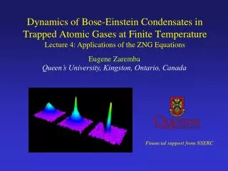
Lecture 4: Applications of the ZNG Equations. Dynamics of Bose-Einstein Condensates in Trapped Atomic Gases at Finite Temperature. Queen’s University, Kingston, Ontario, Canada. Eugene Zaremba. Financial support from NSERC. Outline, cont’d. Lecture 3: Solution of the ZNG Equations.

E N D
Lecture 4: Applications of the ZNG Equations Dynamics of Bose-Einstein Condensates in Trapped Atomic Gases at Finite Temperature Queen’s University, Kingston, Ontario, Canada Eugene Zaremba Financial support from NSERC
Outline, cont’d Lecture 3: Solution of the ZNG Equations • numerical solution of the GGP, split-operator method • numerical solution of the kinetic equation, test-particle method, collision algorithm • model of condensate growth • the moment method, scissors mode and ZNG simulations • the static thermal cloud approximation, dissipative GP equations Lecture 4: Application of the ZNG Equations • quadrupole modes: JILA and ENS experiments • Landau damping: example of monopole (breathing) mode • introduction to vortices • stirring, rotating frames of reference • vortex energetics • phenomenological nucleation and equilibration of vortices • ZNG simulations of vortex precession and relaxation
Quadrupole Modes in Axisymmetric Traps • as our first example we will consider the experimental results obtained by the JILA group for the quadrupole collective modes • a trap anisotropy couples the lowest monopole (l = 0, m = 0) and quadrupole (l = 2, m = 0) modes of an isotropic trap, giving rise to two m = 0 modes with frequencies (Stringari, 1996) E: Derive this result from the quantum hydrodynamic equations in the TF limit using the moment method. Hint: Consider the moment <x2 + y2>. The lower frequency ω− mode corresponds to the m = 0 mode of interest in the experiments. For the experimental value of λ = √8, this mode has the frequency . The other mode of interest is the m = 2 quadrupole mode with frequency . • above TBEC the thermal cloud undergoes a breathing-like oscillation at the frequency .
Visualizing the Modes m = 0 m = 2
Exciting the Modes in the ZNG Simulations • as a model, we start with the equilibrium configuration and impose velocities on the two components: m = 2 m = 0 • for the condensate, this is done by multiplying the equilibrium wavefunction by an appropriate phase factor; for the thermal cloud we simply add a small position-dependent velocity to each test particle
Model Results • the points with error bars are experimental results • the blue squares are the results obtained when only the condensate is excited • the triangles are the results for excitation of both the condensate and thermal cloud. The blue triangles are for the condensate and the red triangles are for the thermal cloud. • the results for m = 0 are poor at the higher temperatures T/TBEC
Experimental Excitation Scheme • we now show what happens when the actual experimental excitation scheme is used for the m = 0 mode: the transverse frequency is modulated harmonically for a short interval • this panel shows the condensate quadrupole moment; the vertical lines indicate the experimental observation window • this panel shows the thermal cloud quadrupole moment = 1.95 T/TBEC = 0.8
Frequencies and Damping Rates Drive Frequencies • when the drive frequency approaches the thermal cloud resonance at 2, the thermal cloud mean field drives the condensate at its frequency and leads to the upward shift of the condensate frequency at the higher temperatures T/TBEC
The ENS Experiment • “top hat” excitation scheme of the m = 0 transverse breathing mode
Transverse Breathing Mode • for the pure condensate at T = 0, this mode approaches 2 as • for T > TBEC, the thermal cloud in the near-collisionless regime has a transverse-breathing-mode also at 2. This near degeneracy of the condensate and thermal cloud modes has an important consequence. T = 125 nK • shown are the results of a ZNG simulation with the top-hat excitation; the red curve is for the condensate and the blue curve is for the thermal cloud
Comparison with Experiment • there is overall good agreement between experiment and theory for both the frequency and damping of the mode • note in particular that the damping rate is an order of magnitude smaller than found in the JILA experiments; the obvious question is: Why?
Further Simulation Results • in this simulation, all collisions are switched off; evidently, damping is a collisional effect • this is a simulation of the m = 2 mode; the damping is much stronger than for the transverse breathing mode. In addition, the damping persists even when collisions are switched off. This damping mechanism – Landau damping – is usually the dominant damping mechanism
Landau Damping • we have seen earlier that the source of damping in the static thermal cloud approximation is the collisional exchange of atoms between the condensate and thermal cloud • in the case of the transverse breathing mode in elongated traps, collisions within the thermal cloud are responsible for the damping • however, in many cases, condensate modes decay predominantly as a result of Landau damping; in the context of the GGP equation, it arises from the mean-field interaction with the thermal cloud • this mean-field interaction effectively exerts a force on the condensate; conversely, the condensate exerts a force on the thermal cloud. This force can do work on the thermal cloud and in this way transfer energy to it. Interestingly, in order for the effect of the thermal cloud on the condensate to be accounted for properly, the detailed dynamical evolution of the thermal cloud density is required.
Comparison of Damping Mechanisms: The Monopole Mode • in these simulations we consider 5 × 10⁴ 87Rb atoms in an isotropic trap; the monopole, or radial breathing mode is excited by a radial scaling of the equilibrium condensate wavefunction: T/TBEC = 0.65 • the solid curve is the full simulation; the dashed curve neglects collisions • C12 = C22 = 0 (solid circles); C22 only (open circles); all collisions (triangles) • Landau damping dominates up to T≅ 0.6 TBEC
Vortices • one of the most exciting developments in the study of cold atomic gases was the observation of vortices. The reason for this was that the appearance of a vortex was a direct manifestation of the superfluid nature of a Bose-condensed gas. Of course, superfluidity was evident in many other situations not involving vortices (for example, condensate collective modes) but somehow the observation of vortices just had a lot more impact on the imagination of physicists! • one of the early challenges in the cold atom community was creating vortices in the first place – it was a kind of holy grail! But ironically, once the tricks had been learned, vortices could be created at will and in abundance. • although much has been learned, there are still unanswered questions regarding the creation of vortices, how they equilibrate and how they behave. I will be addressing some of these questions in the following.
GP Description of Quantized Vortices • to begin, let’s consider a line vortex in a uniform condensate at zero temperature. What we are looking for is a specific solution of the time-independent GP equation having the form • as opposed to the earlier examples we have considered, this stationary state is complex and thus has a velocity field associated with it: • this velocity field is irrotational except along the line of the vortex where • as a result there is a quantized circulation given by • the integer l is sometimes referred to as the ‘charge’ of the vortex; the most stable vortex is singly-quantized
GP Description of Quantized Vortices, cont’d • because the velocity field diverges at ρ = 0, the radial part of the wavefunction must vanish – the vortex has a core • the size of the core is determined by the healing length • the vortex state is an excited state solution of the GP equation and this state has a higher energy. One would therefore not expect to see vortices in an equilibrium situation. This is true unless the condensate is stirred.
Stirring • in order to create vortices, one must impart some angular momentum to the system; this can be done by imposing a rotating anisotropic external potential • in the rotating frame • in the lab frame E: Show that this potential is time independent if ε = 0. • the potential is static in the rotating frame, but this frame is a noninertial frame of reference – both classical and quantum equations of motion are different in the two frames of reference
Rotating Frames of Reference: Classical Treatment • the classical equation of motion for a particle in the rotating frame is • this equation corresponds to the Hamiltonian • the distribution function in this frame is then found to satisfy • the steady-state equilibrium solution is with
Rotating Frames of Reference: Classical Treatment, cont’d • since p’ = pand v = v’ + Ω x r’, we see that p’ – mvrb = mv’, that is the velocity distribution is isotropic in the rotating frame • this same distribution in the lab frame is • this shows that the velocity field in the lab frame is v(r) = vrb = Ω x rwhich implies that the density distribution rotates rigidly with angular velocity Ω. The centrifugal potential Vcent causes the density to bulge out in the radial direction
Rotating Frames of Reference: Quantum Treatment • similar results are found in the quantum treatment. Without going into details (see Ch. 9 of GNZ), one finds that the state vector in the lab frame is given by where • this state vector is defined by a time-independent trapping potential but now the angular velocity appears together with the angular momentum operator. The physical state in the lab frame is obtained by performing an active rotation of the state through an angle Ωt. • if we look for stationary states in the rotating frame, these states are affected by the angular momentum term in the Hamiltonian. The ground state will depend on the magnitude of Ω and if Ω is sufficiently large, the ground state will contain vortices.
Vortex Energetics at the GP Level • we now consider the relative stability of a single axial vortex in a trapped gas at T = 0 relative to the vortex-free state. In the rotating frame the GP energy functionalis • the energy difference between the vortex-free state and the single-vortex configuration is • where one finds in the TF approximation that • this defines a critical angular velocity above which the vortex is thermodynamically stable
Vortex Energetics at the GP Level, cont’d • similar calculations can be carried out for an off-centre vortex (Fetter and Svidzinsky, 2001) • for Ω = 0 (a), the energy of the vortex decreases as it moves to the edge of the cloud; if there were some way to dissipate the energy, the vortex would move to the edge and be expelled from the condensate. The curve (c) corresponds to the situation where the vortex at the centre of the trap is thermodynamically stable.
GP Solutions for a Rotating Anisotropic Trap • at low rotation rates, the flow is irrotational: (a) flow in lab frame, (b) flow in rotating frame (Feder et al., 1999) • the simulations use imaginary time propagation to find the ground state in the rotating frame; the number of vortices is seen to increase with Ω • in the lab frame these images would rotate with an angular velocity Ω
Vortex Nucleation: 2D Simulations • the stirring of a nearly pure condensate leads to the formation of vortices. The nucleation process is of considerable interest and can be simulated using a phenomenological dissipative GP equation of the kind developed earlier: • these 2D simulations were performed by Tsubota et al., 2002 • starting with an isotropic state, a rotating anisotropic potential is switched on; one observes a quadrupole distortion (b), excitation of surface modes (c), penetration of vortices (d-e) and equilibration (f)
Vortex Nucleation: 3D Simulations • the following animation was provided by Naramisa Sasa • the same dissipative GP equation was used for these simulations with a constant dissipation constant ; as we have seen, this parameter can be related to the collisional exchange of atoms between the condensate and thermal cloud • all these results are at the level of the static thermal cloud approximation which ignores the dynamics of the thermal cloud
Vortex Precession • these experimental images (and fits) show the precession of an off-center vortex, Anderson et al., PRL 85, 2857 (2000) • the sense of precession can be understood by appealing to image theory of superfluid flow • the image vortex has the opposite sense of circulation to ensure that the normal current vanishes at the boundary • the flow field of the image sweeps the vortex along the surface in the direction shown
Vortex Precession, cont’d • at T =0, the dynamics is conservative and the vortex precesses at a constant radius • a Lagrangian analysis (Lundh and Ao, Fetter and Svidzinsky) gives a precession frequency of • Bogoliubov theory for a condensate with a central vortex gives condensate modes with (Dodd et al., PRA 56, 587 (1997)) • the so-called anomalous m = −1 mode has a negative frequency and • this mode corresponds to the precession of an off-centre vortex (Fetter and Svidzinsky) and has the same sense of precession as that of the vortex
Vortex Precession at Finite T in the HFBP Theory • shown below is the condensate and thermal cloud densities as calculated in the HFBP approximation • the m = −1 mode has a frequency −1 > 0: thus thesense of precession is opposite to the T = 0 case • dynamics is equivalent to the condensate moving in the static external potential • the thermal cloud density acts as a pinning centre and causes the opposite sense of precession: this is analogous the the violation of the Kohn theorem in the HFBP for the c.m. dipole mode • to restore the proper behaviour one must treat the dynamics of the thermal cloud in a consistent fashion; this is what the ZNG theory provides
ZNG Simulation of Vortex Precession • starting with a vortex-free equilibrium state at a given temperature T, the vortex state is obtained by multiplying the condensate wavefunction by the phase factor exp[iS(r)] where • this imprints the velocity field of a straight vortex at (x0, y0) • the GP equation is then evolved in imaginary time for a short period until a fully-developed vortex state in the condensate is formed • this initial state is a quasi-equilibrium state containing one off-centre vortex • the dynamics of the vortex is then obtained by evolving the full set of ZNG equations in real time
Vortex Decay* • at finite temperatures, an off-centre vortex spirals outwards as its energy is dissipated due to friction with the thermal cloud • the decay rate is found by fitting the data to an exponential function *Jackson, Proukakis, Barenghi and Zaremba, Phys. Rev. A 79, 053615 (2009)
Condensate and Thermal Cloud Densities • the top panel shows the condensate density; the vortex core with its depleted density appears as a blue dot • the lower panel shows the thermal cloud density; the density has a peak (red) in the vortex core due to the reduced mean-field repulsion from the condensate • the sense of precession is the same as at T = 0
Rotating Thermal Clouds • we now consider a situation in which the thermal cloud undergoes solid-body rotation with angular velocity th. This is achieved by adding vn = thrv to the velocity of each thermal atom in the equilibrium state. There is now a motion of the vortex relative to the thermal cloud. • radial position vs. time: th/v = -0.2 (black), 0 (red), 0.2 (green) 0.37 (blue); T/Tc = 0.7 • decay rate vs.th
Vortex Lattice Formation and Decay* • following an initial stirring phase, the vortices are seen to equilibrate into a triangular lattice; the number of vortices then decays as a function of time *Abo-Shaeer et al., Science 292 (2001)
Decay of Vortex Lattices* • rotating (a) condensate and (b) thermal cloud • aspect ratio for a rotating cloud is • (a) aspect ratio vs. time and (b) rotation rate vs. time *Abo-Shaeer et al., Science 292 (2001)
Decay of Vortex Lattices: Simulations • the figure below shows the evolution for two different initial vortex structures containing 7 vortices (T/Tc = 0.7) • the top panel shows that the outer vortices are shed while the central vortex persists for much longer times; this is in accord with observations • in the lower panel, all vortices are shed; however, for this initial configuration a central, long-lived vortex may still appear
Overview • the ZNG equations provide a reasonably complete description of the dynamics of a Bose-condensed gas at finite temperature • the theory is based on the idea of Bose broken symmetry – it assumes that the condensate exists as a well-defined physical entity even in highly nonequilibrium situations • the thermal cloud can be viewed in (semi-)classical terms as a collection of particle-like excitations • this picture conforms to what we SEE in experiments! • the theory of course is approximate and has its limitations. It is ‘correct’ to the extent that it explains experimental observations. • it is not a theory one would want to apply to highly correlated systems such as atoms in an optical lattice with a few particles per site Quo vadis ZNG? • perhaps Bose mixtures and spinor condensates, dipolar systems, strongly perturbed Bose condensates, …?